makeMoE: 从零开始实现稀疏专家混合语言模型


TL;DR:本博客将逐步介绍如何从零开始实现一个稀疏专家混合语言模型。这篇博客的灵感主要来自于 Andrej Karpathy 的项目“makemore”,并借鉴了该实现中的许多可重用组件。与 makemore 一样,makeMoE 也是一个自回归字符级语言模型,但它使用了上述的稀疏专家混合架构。博客的其余部分将重点介绍该架构的关键元素以及它们的实现方式。我的目标是让您在阅读完这篇博客并逐步查看代码库中的代码后,能够直观地理解它的工作原理。
GitHub 仓库在此处提供端到端实现:https://github.com/AviSoori1x/makeMoE/tree/main

随着 Mixtral 的发布以及 GPT-4 可能是一个专家混合大型语言模型的说法,人们对这种模型架构产生了浓厚的兴趣。然而,在稀疏专家混合语言模型中,大部分组件与传统 Transformer 共享。尽管看似简单,但经验证据表明,训练稳定性是这些模型的主要问题之一。像这样的可修改小规模实现可能有助于快速试验新方法。
在此次实现中,我对 makemore 架构进行了一些重大修改:
- 稀疏专家混合代替了单一的前馈神经网络。
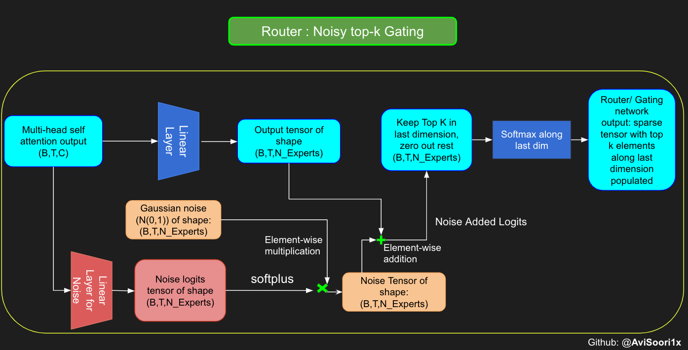
- Top-k 门控和带噪声的 Top-k 门控实现。
- 初始化 - 此处使用 Kaiming He 初始化,但本 Notebook 的重点是可修改性,因此您可以换用 Xavier/Glorot 初始化等进行尝试。
然而,以下内容与 makemore 保持不变:
- 数据集、预处理(分词)以及 Andrej 最初选择的语言建模任务——生成类似莎士比亚的文本。
- 因果自注意力实现
- 训练循环
- 推理逻辑
我们开始吧!
稀疏专家混合语言模型,正如预期的那样,依赖于自注意力机制进行上下文理解。接下来,我们将深入探讨专家混合模块的复杂性。首先,让我们深入了解自注意力以刷新我们的理解。
理解因果缩放点积自注意力的直觉
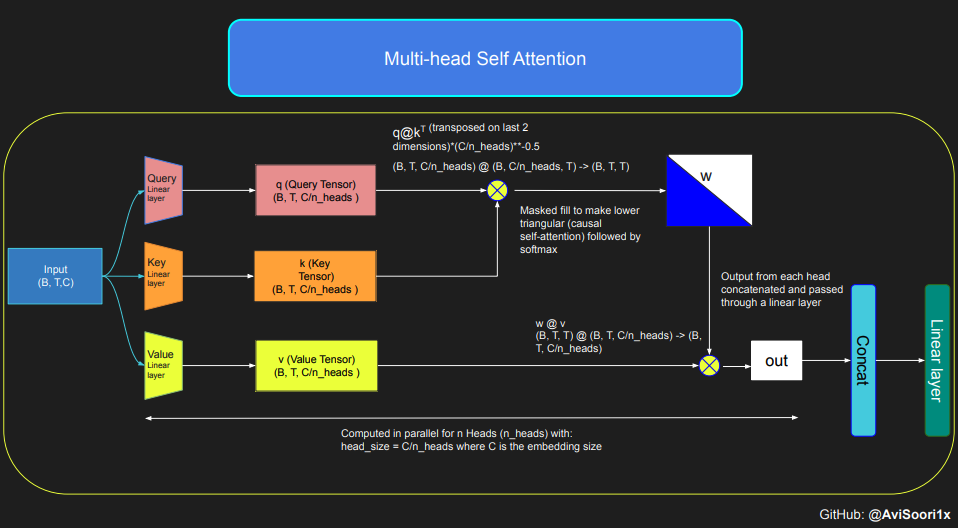
所提供的代码演示了自注意力的机制和基本概念,特别关注经典的缩放点积自注意力。在此变体中,查询、键和值矩阵都源自相同的输入序列。为了确保自回归语言生成过程的完整性,特别是在仅解码器模型中,代码实现了掩码。这种掩码技术至关重要,因为它会遮盖当前标记位置之后的所有信息,从而将模型的注意力仅引导到序列的先前部分。这种注意力机制被称为因果自注意力。值得注意的是,稀疏专家混合模型不限于仅解码器 Transformer 架构。事实上,该领域的大部分重要工作,特别是 Shazeer 等人的工作,都围绕 T5 架构,该架构包含 Transformer 模型中的编码器和解码器组件。
#This code is borrowed from Andrej Karpathy's makemore repository linked in the repo.
The self attention layers in Sparse mixture of experts models are the same as
in regular transformer models

torch.manual_seed(1337)
B,T,C = 4,8,32 # batch, time, channels
x = torch.randn(B,T,C)

# let's see a single Head perform self-attention
head_size = 16
key = nn.Linear(C, head_size, bias=False)
query = nn.Linear(C, head_size, bias=False)
value = nn.Linear(C, head_size, bias=False)
k = key(x)   # (B, T, 16)
q = query(x) # (B, T, 16)
wei =  q @ k.transpose(-2, -1) # (B, T, 16) @ (B, 16, T) ---> (B, T, T)

tril = torch.tril(torch.ones(T, T))
#wei = torch.zeros((T,T))
wei = wei.masked_fill(tril == 0, float('-inf'))
wei = F.softmax(wei, dim=-1) #B,T,T

v = value(x) #B,T,H
out = wei @ v # (B,T,T) @ (B,T,H) -> (B,T,H)
out.shape
torch.Size([4, 8, 16])
因果自注意力与多头因果自注意力的代码可以组织如下。多头自注意力并行应用多个注意力头,每个头关注通道(嵌入维度)的不同部分。多头自注意力由于其固有的并行实现,本质上改进了学习过程并提高了模型训练效率。请注意,我在整个实现中使用了 dropout 进行正则化,即防止过拟合。
#Causal scaled dot product self-Attention Head
n_embd = 64
n_head = 4
n_layer = 4
head_size = 16
dropout = 0.1

class Head(nn.Module):
    """ one head of self-attention """

    def __init__(self, head_size):
        super().__init__()
        self.key = nn.Linear(n_embd, head_size, bias=False)
        self.query = nn.Linear(n_embd, head_size, bias=False)
        self.value = nn.Linear(n_embd, head_size, bias=False)
        self.register_buffer('tril', torch.tril(torch.ones(block_size, block_size)))

        self.dropout = nn.Dropout(dropout)

    def forward(self, x):
        B,T,C = x.shape
        k = self.key(x)   # (B,T,C)
        q = self.query(x) # (B,T,C)
        # compute attention scores ("affinities")
        wei = q @ k.transpose(-2,-1) * C**-0.5 # (B, T, C) @ (B, C, T) -> (B, T, T)
        wei = wei.masked_fill(self.tril[:T, :T] == 0, float('-inf')) # (B, T, T)
        wei = F.softmax(wei, dim=-1) # (B, T, T)
        wei = self.dropout(wei)
        # perform the weighted aggregation of the values
        v = self.value(x) # (B,T,C)
        out = wei @ v # (B, T, T) @ (B, T, C) -> (B, T, C)
        return out
多头自注意力实现如下
#Multi-Headed Self Attention
class MultiHeadAttention(nn.Module):
    """ multiple heads of self-attention in parallel """

    def __init__(self, num_heads, head_size):
        super().__init__()
        self.heads = nn.ModuleList([Head(head_size) for _ in range(num_heads)])
        self.proj = nn.Linear(n_embd, n_embd)
        self.dropout = nn.Dropout(dropout)

    def forward(self, x):
        out = torch.cat([h(x) for h in self.heads], dim=-1)
        out = self.dropout(self.proj(out))
        return out
创建一个专家模块,即一个简单的多层感知器
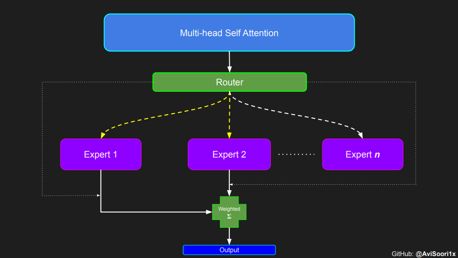
在稀疏专家混合(MoE)架构中,每个 Transformer 块内的自注意力机制保持不变。然而,每个块的结构发生了一个显著变化:标准的 Feed-forward 神经网络被替换为几个稀疏激活的 Feed-forward 网络,这些网络被称为专家。“稀疏激活”指的是序列中的每个 token 只被路由到这些专家中的有限数量——通常是一到两个——而不是全部可用专家。这有助于训练和推理速度,因为在每次前向传播中只激活少数专家。然而,所有专家都必须驻留在 GPU 内存中,当总参数量达到数千亿甚至数万亿时,这会带来有趣的部署问题。
#Expert module
class Expert(nn.Module):
    """ An MLP is a simple linear layer followed by a non-linearity i.e. each Expert """

    def __init__(self, n_embd):
        super().__init__()
        self.net = nn.Sequential(
            nn.Linear(n_embd, 4 * n_embd),
            nn.ReLU(),
            nn.Linear(4 * n_embd, n_embd),
            nn.Dropout(dropout),
        )

    def forward(self, x):
        return self.net(x)
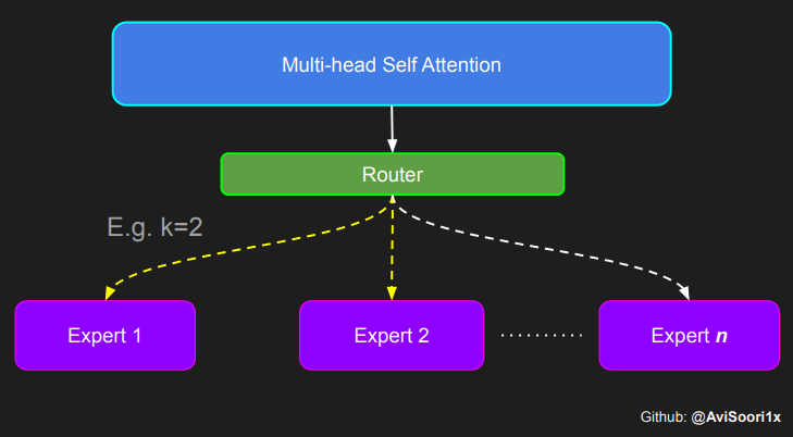
通过示例理解 Top-k 门控的直觉
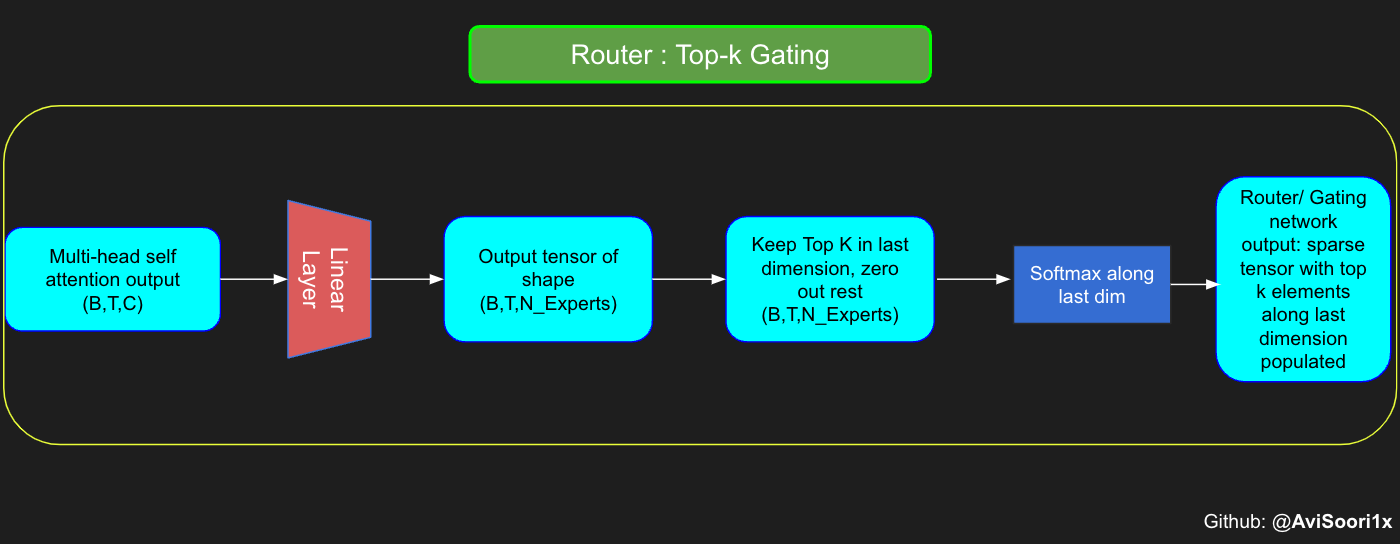
门控网络,也称为路由器,决定了哪个专家网络接收来自多头注意力的每个 token 的输出。让我们考虑一个简单的例子:假设有 4 个专家,并且 token 将被路由到前 2 个专家。最初,我们通过线性层将 token 输入到门控网络。该层将输入张量从 (2, 4, 32) 的形状(表示批处理大小、标记、n_embed,其中 n_embed 是输入的通道维度)投影到 (2, 4, 4) 的新形状,这对应于(批处理大小、标记、专家数量),其中专家数量是专家网络的数量。在此之后,我们确定沿最后一个维度的前 k=2 个最高值及其各自的索引。
#Understanding how gating works
num_experts = 4
top_k=2
n_embed=32


#Example multi-head attention output for a simple illustrative example, consider n_embed=32, context_length=4 and batch_size=2
mh_output = torch.randn(2, 4, n_embed)

topkgate_linear = nn.Linear(n_embed, num_experts) # nn.Linear(32, 4)

logits = topkgate_linear(mh_output)
top_k_logits, top_k_indices = logits.topk(top_k, dim=-1)  # Get top-k experts
top_k_logits, top_k_indices
#output:
(tensor([[[ 0.0246, -0.0190],
          [ 0.1991,  0.1513],
          [ 0.9749,  0.7185],
          [ 0.4406, -0.8357]],

         [[ 0.6206, -0.0503],
          [ 0.8635,  0.3784],
          [ 0.6828,  0.5972],
          [ 0.4743,  0.3420]]], grad_fn=<TopkBackward0>),
 tensor([[[2, 3],
          [2, 1],
          [3, 1],
          [2, 1]],

         [[0, 2],
          [0, 3],
          [3, 2],
          [3, 0]]]))
通过仅保留沿最后一个维度中各自索引的前 k 个值来获得稀疏门控输出。其余部分填充为“-inf”,并通过 softmax 激活。这将“-inf”值推向零,使前两个值更加突出并和为 1。这个和为 1 有助于专家输出的加权。
zeros = torch.full_like(logits, float('-inf')) #full_like clones a tensor and fills it with a specified value (like infinity) for masking or calculations.
sparse_logits = zeros.scatter(-1, top_k_indices, top_k_logits)
sparse_logits
#output
tensor([[[   -inf,    -inf,  0.0246, -0.0190],
         [   -inf,  0.1513,  0.1991,    -inf],
         [   -inf,  0.7185,    -inf,  0.9749],
         [   -inf, -0.8357,  0.4406,    -inf]],

        [[ 0.6206,    -inf, -0.0503,    -inf],
         [ 0.8635,    -inf,    -inf,  0.3784],
         [   -inf,    -inf,  0.5972,  0.6828],
         [ 0.3420,    -inf,    -inf,  0.4743]]], grad_fn=<ScatterBackward0>)
gating_output= F.softmax(sparse_logits, dim=-1)
gating_output
#ouput
tensor([[[0.0000, 0.0000, 0.5109, 0.4891],
         [0.0000, 0.4881, 0.5119, 0.0000],
         [0.0000, 0.4362, 0.0000, 0.5638],
         [0.0000, 0.2182, 0.7818, 0.0000]],

        [[0.6617, 0.0000, 0.3383, 0.0000],
         [0.6190, 0.0000, 0.0000, 0.3810],
         [0.0000, 0.0000, 0.4786, 0.5214],
         [0.4670, 0.0000, 0.0000, 0.5330]]], grad_fn=<SoftmaxBackward0>)
泛化和模块化上述代码,并为负载均衡添加带噪声的 Top-k 门控
# First define the top k router module
class TopkRouter(nn.Module):
    def __init__(self, n_embed, num_experts, top_k):
        super(TopkRouter, self).__init__()
        self.top_k = top_k
        self.linear =nn.Linear(n_embed, num_experts)

    def forward(self, mh_ouput):
        # mh_ouput is the output tensor from multihead self attention block
        logits = self.linear(mh_output)
        top_k_logits, indices = logits.topk(self.top_k, dim=-1)
        zeros = torch.full_like(logits, float('-inf'))
        sparse_logits = zeros.scatter(-1, indices, top_k_logits)
        router_output = F.softmax(sparse_logits, dim=-1)
        return router_output, indices
让我们用一些样本输入来测试功能
#Testing this out:
num_experts = 4
top_k = 2
n_embd = 32

mh_output = torch.randn(2, 4, n_embd)  # Example input
top_k_gate = TopkRouter(n_embd, num_experts, top_k)
gating_output, indices = top_k_gate(mh_output)
gating_output.shape, gating_output, indices
#And it works!!
#output
(torch.Size([2, 4, 4]),
 tensor([[[0.5284, 0.0000, 0.4716, 0.0000],
          [0.0000, 0.4592, 0.0000, 0.5408],
          [0.0000, 0.3529, 0.0000, 0.6471],
          [0.3948, 0.0000, 0.0000, 0.6052]],

         [[0.0000, 0.5950, 0.4050, 0.0000],
          [0.4456, 0.0000, 0.5544, 0.0000],
          [0.7208, 0.0000, 0.0000, 0.2792],
          [0.0000, 0.0000, 0.5659, 0.4341]]], grad_fn=<SoftmaxBackward0>),
 tensor([[[0, 2],
          [3, 1],
          [3, 1],
          [3, 0]],

         [[1, 2],
          [2, 0],
          [0, 3],
          [2, 3]]]))
尽管最近发布的 Mixtral 论文并未提及,但我相信带噪声的 top-k 门控是训练 MoE 模型的重要工具。本质上,你不想让所有 token 都发送到同一组“偏爱”的专家。你需要一个精细的探索与利用平衡。为此,为了负载均衡,向门控线性层的 logits 添加标准正态噪声会很有帮助。这使得训练更有效率。
#Changing the above to accomodate noisy top-k gating
class NoisyTopkRouter(nn.Module):
    def __init__(self, n_embed, num_experts, top_k):
        super(NoisyTopkRouter, self).__init__()
        self.top_k = top_k
        #layer for router logits
        self.topkroute_linear = nn.Linear(n_embed, num_experts)
        self.noise_linear =nn.Linear(n_embed, num_experts)


    def forward(self, mh_output):
        # mh_ouput is the output tensor from multihead self attention block
        logits = self.topkroute_linear(mh_output)

        #Noise logits
        noise_logits = self.noise_linear(mh_output)

        #Adding scaled unit gaussian noise to the logits
        noise = torch.randn_like(logits)*F.softplus(noise_logits)
        noisy_logits = logits + noise

        top_k_logits, indices = noisy_logits.topk(self.top_k, dim=-1)
        zeros = torch.full_like(noisy_logits, float('-inf'))
        sparse_logits = zeros.scatter(-1, indices, top_k_logits)
        router_output = F.softmax(sparse_logits, dim=-1)
        return router_output, indices
让我们再测试一下这个实现
#Testing this out, again:
num_experts = 8
top_k = 2
n_embd = 16

mh_output = torch.randn(2, 4, n_embd)  # Example input
noisy_top_k_gate = NoisyTopkRouter(n_embd, num_experts, top_k)
gating_output, indices = noisy_top_k_gate(mh_output)
gating_output.shape, gating_output, indices
#It works!!
#output
(torch.Size([2, 4, 8]),
 tensor([[[0.4181, 0.0000, 0.5819, 0.0000, 0.0000, 0.0000, 0.0000, 0.0000],
          [0.4693, 0.5307, 0.0000, 0.0000, 0.0000, 0.0000, 0.0000, 0.0000],
          [0.0000, 0.4985, 0.5015, 0.0000, 0.0000, 0.0000, 0.0000, 0.0000],
          [0.0000, 0.0000, 0.0000, 0.2641, 0.0000, 0.7359, 0.0000, 0.0000]],

         [[0.0000, 0.0000, 0.0000, 0.6301, 0.0000, 0.3699, 0.0000, 0.0000],
          [0.0000, 0.0000, 0.0000, 0.4766, 0.0000, 0.0000, 0.0000, 0.5234],
          [0.0000, 0.0000, 0.0000, 0.6815, 0.0000, 0.0000, 0.3185, 0.0000],
          [0.4482, 0.5518, 0.0000, 0.0000, 0.0000, 0.0000, 0.0000, 0.0000]]],
        grad_fn=<SoftmaxBackward0>),
 tensor([[[2, 0],
          [1, 0],
          [2, 1],
          [5, 3]],

         [[3, 5],
          [7, 3],
          [3, 6],
          [1, 0]]]))
创建一个稀疏专家混合模块
此过程的主要方面涉及门控网络的输出。在获得这些结果后,将 top k 值与给定 token 的相应 top-k 专家输出进行选择性相乘。这种选择性相乘形成一个加权和,构成 SparseMoe 块的输出。此过程的关键和挑战部分是避免不必要的乘法。必须仅对 top_k 专家进行前向传播,然后计算此加权和。对每个专家进行前向传播将违背使用稀疏 MoE 的目的,因为它将不再是稀疏的。
class SparseMoE(nn.Module):
    def __init__(self, n_embed, num_experts, top_k):
        super(SparseMoE, self).__init__()
        self.router = NoisyTopkRouter(n_embed, num_experts, top_k)
        self.experts = nn.ModuleList([Expert(n_embed) for _ in range(num_experts)])
        self.top_k = top_k

    def forward(self, x):
        gating_output, indices = self.router(x)
        final_output = torch.zeros_like(x)

        # Reshape inputs for batch processing
        flat_x = x.view(-1, x.size(-1))
        flat_gating_output = gating_output.view(-1, gating_output.size(-1))

        # Process each expert in parallel
        for i, expert in enumerate(self.experts):
            # Create a mask for the inputs where the current expert is in top-k
            expert_mask = (indices == i).any(dim=-1)
            flat_mask = expert_mask.view(-1)

            if flat_mask.any():
                expert_input = flat_x[flat_mask]
                expert_output = expert(expert_input)

                # Extract and apply gating scores
                gating_scores = flat_gating_output[flat_mask, i].unsqueeze(1)
                weighted_output = expert_output * gating_scores

                # Update final output additively by indexing and adding
                final_output[expert_mask] += weighted_output.squeeze(1)

        return final_output
使用示例输入测试上述实现是否有效很有帮助。运行以下代码后,我们可以看到它确实有效!
import torch
import torch.nn as nn

#Let's test this out
num_experts = 8
top_k = 2
n_embd = 16
dropout=0.1

mh_output = torch.randn(4, 8, n_embd)  # Example multi-head attention output
sparse_moe = SparseMoE(n_embd, num_experts, top_k)
final_output = sparse_moe(mh_output)
print("Shape of the final output:", final_output.shape)
Shape of the final output: torch.Size([4, 8, 16])
需要强调的是,重要的是要认识到,如上图所示,来自路由器/门控网络的 top_k 专家输出的幅值也至关重要。这些 top_k 索引标识了被激活的专家,而这些 top_k 维度中值的幅值决定了它们各自的权重。加权求和的概念在下图中得到了进一步强调。
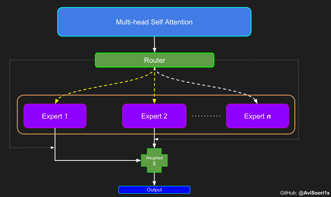
将所有内容整合在一起
多头自注意力和稀疏专家混合被组合起来,形成一个稀疏专家混合 Transformer 块。就像在普通 Transformer 块中一样,添加了跳跃连接以确保训练稳定并避免梯度消失等问题。此外,还采用了层归一化来进一步稳定学习过程。
#Create a self attention + mixture of experts block, that may be repeated several number of times
class Block(nn.Module):
    """ Mixture of Experts Transformer block: communication followed by computation (multi-head self attention + SparseMoE) """

    def __init__(self, n_embed, n_head, num_experts, top_k):
        # n_embed: embedding dimension, n_head: the number of heads we'd like
        super().__init__()
        head_size = n_embed // n_head
        self.sa = MultiHeadAttention(n_head, head_size)
        self.smoe = SparseMoE(n_embed, num_experts, top_k)
        self.ln1 = nn.LayerNorm(n_embed)
        self.ln2 = nn.LayerNorm(n_embed)

    def forward(self, x):
        x = x + self.sa(self.ln1(x))
        x = x + self.smoe(self.ln2(x))
        return x
最后,将所有内容整合在一起,以创建一个稀疏专家混合语言模型。
class SparseMoELanguageModel(nn.Module):

    def __init__(self):
        super().__init__()
        # each token directly reads off the logits for the next token from a lookup table
        self.token_embedding_table = nn.Embedding(vocab_size, n_embed)
        self.position_embedding_table = nn.Embedding(block_size, n_embed)
        self.blocks = nn.Sequential(*[Block(n_embed, n_head=n_head, num_experts=num_experts,top_k=top_k) for _ in range(n_layer)])
        self.ln_f = nn.LayerNorm(n_embed) # final layer norm
        self.lm_head = nn.Linear(n_embed, vocab_size)

    def forward(self, idx, targets=None):
        B, T = idx.shape

        # idx and targets are both (B,T) tensor of integers
        tok_emb = self.token_embedding_table(idx) # (B,T,C)
        pos_emb = self.position_embedding_table(torch.arange(T, device=device)) # (T,C)
        x = tok_emb + pos_emb # (B,T,C)
        x = self.blocks(x) # (B,T,C)
        x = self.ln_f(x) # (B,T,C)
        logits = self.lm_head(x) # (B,T,vocab_size)

        if targets is None:
            loss = None
        else:
            B, T, C = logits.shape
            logits = logits.view(B*T, C)
            targets = targets.view(B*T)
            loss = F.cross_entropy(logits, targets)

        return logits, loss

    def generate(self, idx, max_new_tokens):
        # idx is (B, T) array of indices in the current context
        for _ in range(max_new_tokens):
            # crop idx to the last block_size tokens
            idx_cond = idx[:, -block_size:]
            # get the predictions
            logits, loss = self(idx_cond)
            # focus only on the last time step
            logits = logits[:, -1, :] # becomes (B, C)
            # apply softmax to get probabilities
            probs = F.softmax(logits, dim=-1) # (B, C)
            # sample from the distribution
            idx_next = torch.multinomial(probs, num_samples=1) # (B, 1)
            # append sampled index to the running sequence
            idx = torch.cat((idx, idx_next), dim=1) # (B, T+1)
        return idx
初始化对于深度神经网络的高效训练至关重要。此处使用 Kaiming He 初始化是因为专家中存在 ReLU 激活。欢迎尝试 Glorot 初始化,它在 Transformer 中更常用。Jeremy Howard 的 Fastai Part 2 有一节出色的讲座,从头开始实现了这些内容:https://course.fastai.net.cn/Lessons/lesson17.html。文献中指出 Glorot 初始化通常用于 Transformer 模型,因此这是一个可能改善模型性能的机会。
def kaiming_init_weights(m):
    if isinstance (m, (nn.Linear)):
        init.kaiming_normal_(m.weight)

model = SparseMoELanguageModel()
model.apply(kaiming_init_weights)
我使用 mlflow 来跟踪和记录重要的指标以及训练超参数。我在这里展示的训练循环包含了这些代码。如果您只想在不使用 mlflow 的情况下进行训练,makeMoE github 仓库中的 notebook 包含不带 MLFlow 的代码块。我个人觉得跟踪参数和指标非常方便,尤其是在进行实验时。
#Using MLFlow
m = model.to(device)
# print the number of parameters in the model
print(sum(p.numel() for p in m.parameters())/1e6, 'M parameters')

# create a PyTorch optimizer
optimizer = torch.optim.AdamW(model.parameters(), lr=learning_rate)
#mlflow.set_experiment("makeMoE")
with mlflow.start_run():
    #If you use mlflow.autolog() this will be automatically logged. I chose to explicitly log here for completeness
    params = {"batch_size": batch_size , "block_size" : block_size, "max_iters": max_iters, "eval_interval": eval_interval,
              "learning_rate": learning_rate, "device": device, "eval_iters": eval_iters, "dropout" : dropout, "num_experts": num_experts, "top_k": top_k }
    mlflow.log_params(params)
    for iter in range(max_iters):

        # every once in a while evaluate the loss on train and val sets
        if iter % eval_interval == 0 or iter == max_iters - 1:
            losses = estimate_loss()
            print(f"step {iter}: train loss {losses['train']:.4f}, val loss {losses['val']:.4f}")
            metrics = {"train_loss": losses['train'], "val_loss": losses['val']}
            mlflow.log_metrics(metrics, step=iter)


        # sample a batch of data
        xb, yb = get_batch('train')

        # evaluate the loss
        logits, loss = model(xb, yb)
        optimizer.zero_grad(set_to_none=True)
        loss.backward()
        optimizer.step()
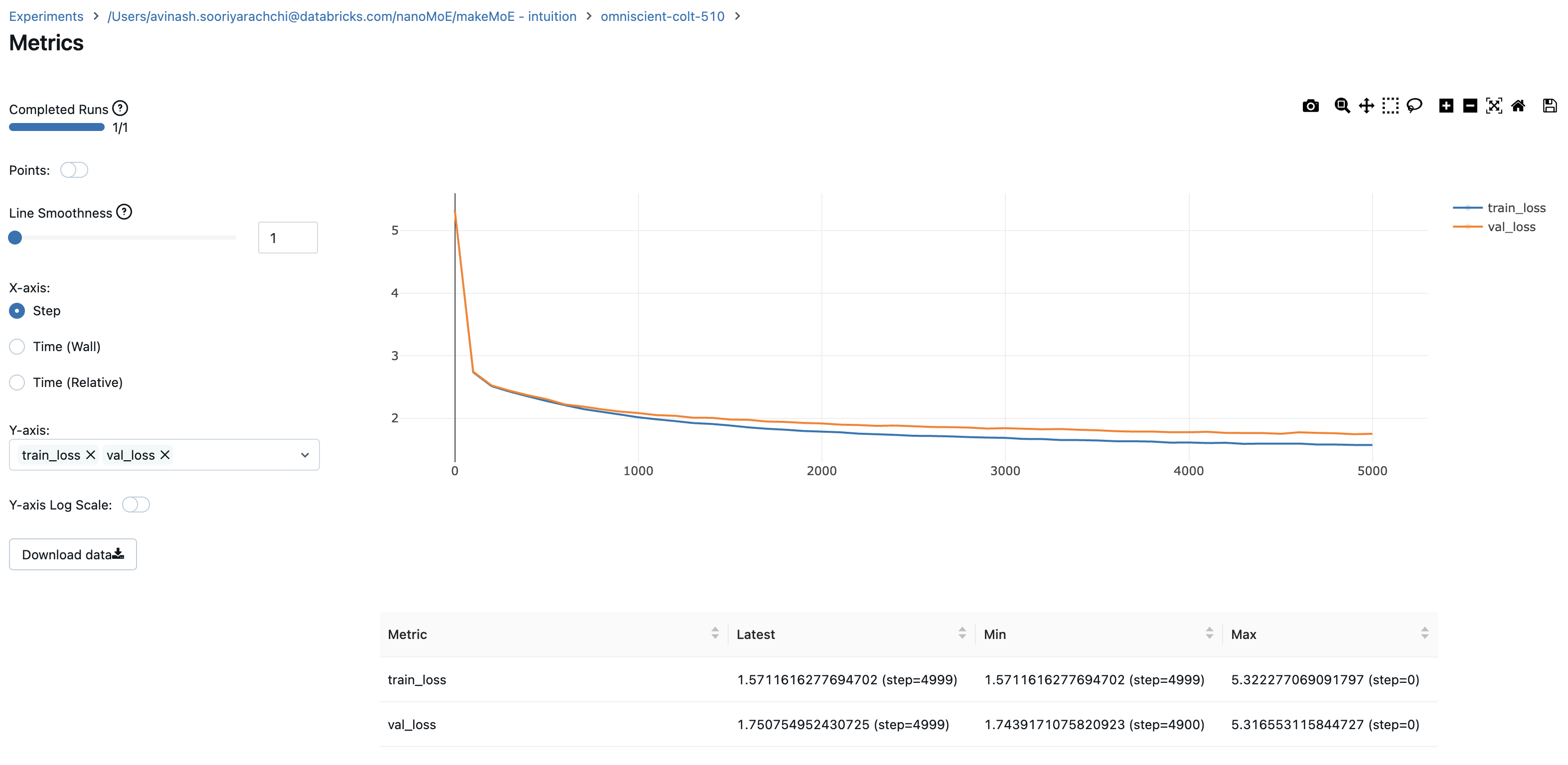
8.996545 M parameters
step 0: train loss 5.3223, val loss 5.3166
step 100: train loss 2.7351, val loss 2.7429
step 200: train loss 2.5125, val loss 2.5233
.
.
.

step 4999: train loss 1.5712, val loss 1.7508
记录训练和验证损失可以很好地指示训练进展。该图显示我可能应该在 4500 步左右停止(当时验证损失略有上升)。
现在我们可以使用这个模型逐个字符地自回归地生成文本。对于一个稀疏激活的约 900 万参数模型,我没有什么可抱怨的。
# generate from the model. Not great. Not too bad either
context = torch.zeros((1, 1), dtype=torch.long, device=device)
print(decode(m.generate(context, max_new_tokens=2000)[0].tolist()))
DUKE VINCENVENTIO:
If it ever fecond he town sue kigh now,
That thou wold'st is steen 't.

SIMNA:
Angent her; no, my a born Yorthort,
Romeoos soun and lawf to your sawe with ch a woft ttastly defy,
To declay the soul art; and meart smad.

CORPIOLLANUS:
Which I cannot shall do from by born und ot cold warrike,
What king we best anone wrave's going of heard and good
Thus playvage; you have wold the grace.
...
我希望这个解释能帮助您理解稀疏专家混合模型架构及其工作原理。
我在这项实现中大量参考了以下出版物:
- Mixtral of experts: https://arxiv.org/pdf/2401.04088.pdf
- Outrageously Large Neural Networks: The Sparsely-Gated Mixture-Of-Experts layer: https://arxiv.org/pdf/1701.06538.pdf
Andrej Karpathy 的原始 makemore 实现
该代码完全在 Databricks 上使用单个 A100 GPU 开发。如果您在 Databricks 上运行此代码,您可以在您选择的云提供商上将它扩展到任意大的 GPU 集群,没有任何问题。我选择使用 MLFlow(Databricks 中预装了它。它是完全开源的,您可以在其他地方轻松地通过 pip 安装),因为我发现它有助于跟踪和记录所有必要的指标。这完全是可选的。请注意,该实现强调可读性和可修改性而不是性能,因此您可以通过多种方式改进它。
鉴于此,这里有一些你可以尝试的事情:
- 使专家混合模块更高效。我相信在上述实现中,对于正确专家的稀疏激活可以进行显著改进。
- 尝试不同的神经网络初始化策略。我列出的来源(Fastai 第二部分)非常棒。
- 从字符级到子词分词
- 对专家数量和 top_k(每个 token 激活的专家数量)进行贝叶斯超参数搜索。这可以粗略地归类为神经网络架构搜索。
- 此处未讨论或实现专家容量。这绝对值得探索。
鉴于人们对专家混合和多模态的兴趣,观察两者交叉领域的发展也将非常有趣。祝您玩得开心!!
PS:本博客的第二部分,包含更高效训练的专家容量实现,请参见此处:https://huggingface.co/blog/AviSoori1x/makemoe2