注解扩散模型


在这篇博客文章中,我们将深入探讨**去噪扩散概率模型**(也称为 DDPM、扩散模型、基于分数的生成模型或简称自编码器),因为研究人员已通过它们在(有)条件图像/音频/视频生成方面取得了卓越的成果。目前(撰写本文时)流行的例子包括 OpenAI 的GLIDE和DALL-E 2,海德堡大学的Latent Diffusion和 Google Brain 的ImageGen。
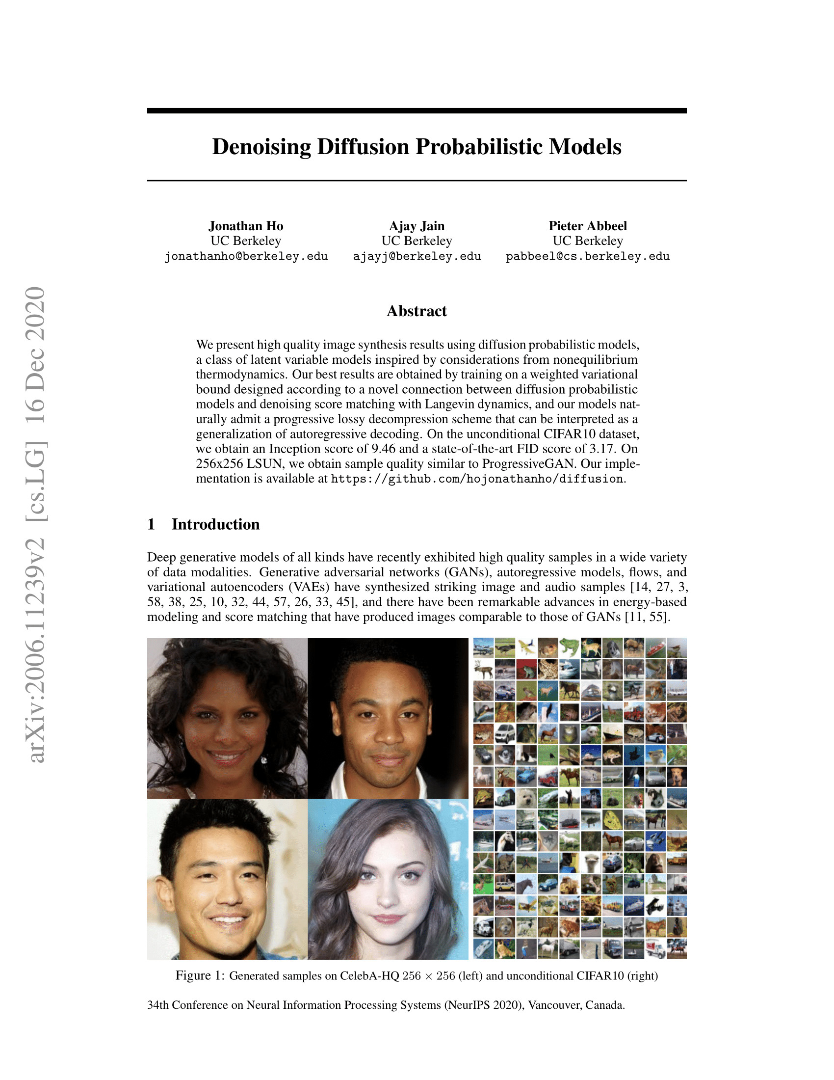
我们将回顾 (Ho 等人,2020) 的原始 DDPM 论文,并根据 Phil Wang 的实现(该实现本身基于原始 TensorFlow 实现)在 PyTorch 中逐步实现它。请注意,用于生成建模的扩散思想实际上在 (Sohl-Dickstein 等人,2015) 中已经提出。然而,直到 (Song 等人,2019)(斯坦福大学)和随后的 (Ho 等人,2020)(Google Brain)独立改进了该方法。
请注意,扩散模型有多种视角。这里,我们采用离散时间(潜在变量模型)的视角,但请务必也查看其他视角。
好的,让我们开始吧!
from IPython.display import Image
Image(filename='assets/78_annotated-diffusion/ddpm_paper.png')
我们首先安装并导入所需的库(假设您已安装 PyTorch)。
!pip install -q -U einops datasets matplotlib tqdm

import math
from inspect import isfunction
from functools import partial

%matplotlib inline
import matplotlib.pyplot as plt
from tqdm.auto import tqdm
from einops import rearrange, reduce
from einops.layers.torch import Rearrange

import torch
from torch import nn, einsum
import torch.nn.functional as F
什么是扩散模型?
去噪扩散模型与其他生成模型(如归一化流、GAN 或 VAE)相比并不复杂:它们都将来自某个简单分布的噪声转换为数据样本。这里也是如此,**神经网络学习从纯噪声开始逐渐去噪数据**。
更具体地针对图像,该设置包含 2 个过程:
- 我们选择的固定(或预定义)正向扩散过程 ,它逐渐向图像添加高斯噪声,直到最终变为纯噪声
- 一个学习到的反向去噪扩散过程 ,其中训练神经网络从纯噪声开始逐渐去噪图像,直到最终得到真实图像。
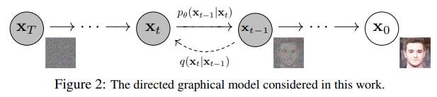
正向和反向过程都由 索引,在有限的时间步长 内进行(DDPM 作者使用 )。您从 开始,从数据分布中采样真实图像 (例如 ImageNet 中的猫图像),并且正向过程在每个时间步长 从高斯分布中采样一些噪声,并将其添加到上一个时间步长的图像中。给定足够大的 和在每个时间步长添加噪声的良好调度,您最终将在 处通过渐进过程得到所谓的各向同性高斯分布。
更数学化的形式
让我们更正式地写下来,因为最终我们需要一个可处理的损失函数,我们的神经网络需要对其进行优化。
令 为真实数据分布,例如“真实图像”。我们可以从这个分布中采样得到图像,。我们定义正向扩散过程 ,它在每个时间步长 根据已知方差调度 添加高斯噪声,如下所示:
回想一下,正态分布(也称为高斯分布)由两个参数定义:均值 和方差 。基本上,每个在时间步长 处的新(略微嘈杂的)图像都从**条件高斯分布**中抽取,其均值为 ,方差为 ,我们可以通过采样 ,然后设置 。
请注意, 在每个时间步长 并不恒定(因此带有下标)——实际上,我们定义了一个所谓的**“方差调度”**,它可以是线性的、二次的、余弦的等等,我们将在后面看到(有点像学习率调度)。
所以从 开始,我们最终得到 ,如果我们将调度设置得当,其中 是纯高斯噪声。
现在,如果知道条件分布 ,那么就可以反向运行该过程:通过采样一些随机高斯噪声 ,然后逐渐“去噪”,最终得到从真实分布 中采样的样本。
但是,我们不知道 。由于它需要知道所有可能图像的分布才能计算这个条件概率,因此它是难以处理的。因此,我们将利用神经网络来**近似(学习)这个条件概率分布**,我们称之为 ,其中 是神经网络的参数,通过梯度下降更新。
好的,所以我们需要一个神经网络来表示反向过程的(条件)概率分布。如果我们假设这个反向过程也是高斯分布,那么回想一下,任何高斯分布都由两个参数定义:
- 一个由 参数化的均值;
- 一个由 参数化的方差;
因此,我们可以将该过程参数化为 ,其中均值和方差也取决于噪声水平 。
因此,我们的神经网络需要学习/表示均值和方差。然而,DDPM 作者决定**固定方差,并让神经网络只学习(表示)这个条件概率分布的均值 **。论文中提到:
首先,我们将 为未训练的时间相关常数。实验表明, 和 (见论文)取得了相似的结果。
这后来在改进扩散模型论文中得到了改进,除了均值之外,神经网络还学习这个反向过程的方差。
所以我们继续,假设我们的神经网络只需要学习/表示这个条件概率分布的均值。
定义目标函数(通过重新参数化均值)
为了推导出学习反向过程均值的目标函数,作者观察到 和 的组合可以看作是一个变分自编码器(VAE)(Kingma 等人,2013)。因此,**变分下界**(也称为 ELBO)可以用于最小化相对于真实数据样本 的负对数似然(我们参考 VAE 论文了解 ELBO 的详细信息)。结果表明,这个过程的 ELBO 是每个时间步长 的损失之和,即 。通过构建正向 过程和反向过程,损失的每一项(除了 )实际上都是**两个高斯分布之间的 KL 散度**,它可以明确地写成关于均值的 L2 损失!
正如 Sohl-Dickstein 等人所示,所构建的正向过程 的直接结果是,我们可以在任何任意噪声水平下根据 采样 (因为高斯分布之和也是高斯分布)。这非常方便:我们不需要重复应用 来采样 。我们有
其中和。我们将此方程称为“良好性质”。这意味着我们可以对高斯噪声进行采样并进行适当缩放,然后将其添加到以直接得到。请注意,是已知方差调度函数的函数,因此也是已知的,可以预先计算。这使得我们能够在训练期间优化损失函数的随机项(换句话说,在训练期间随机采样并优化)。
这个性质的另一个优点是,正如Ho等人所示,可以(经过一些数学推导,我们在此将读者指向这篇优秀博客文章)重新参数化均值,使神经网络学习(预测)添加的噪声(通过网络)用于构成损失的KL项中的噪声水平。这意味着我们的神经网络将成为噪声预测器,而不是(直接的)均值预测器。均值可以计算如下:
最终的目标函数如下所示(对于给定的随机时间步)
这里,是初始(真实,未损坏的)图像,我们看到由固定正向过程给出的直接噪声水平样本。是在时间步采样的纯噪声,而是我们的神经网络。神经网络通过真实噪声和预测高斯噪声之间的简单均方误差 (MSE) 进行优化。
训练算法现在看起来如下:
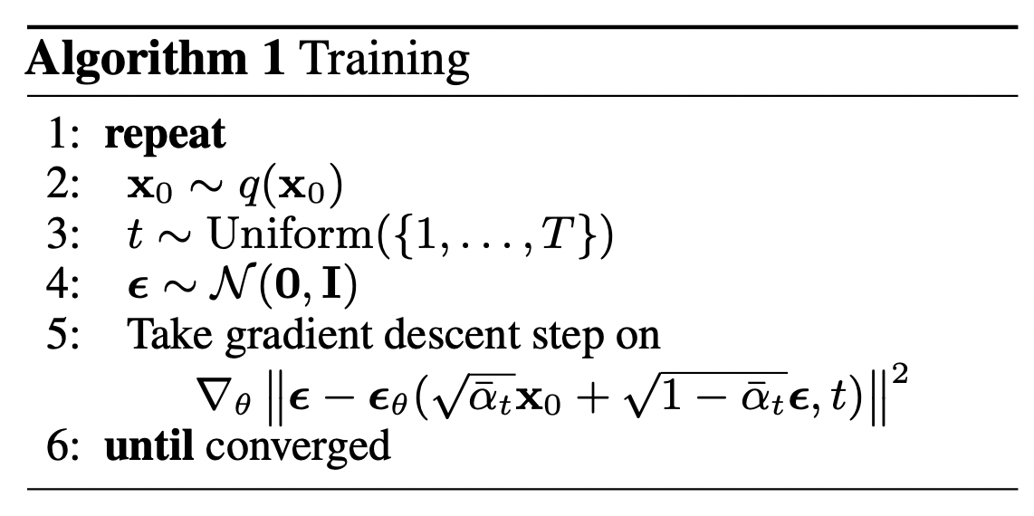
换句话说,
- 我们从真实的未知且可能复杂的数据分布中随机采样一个样本
- 我们从1到均匀采样一个噪声水平(即随机时间步)
- 我们从高斯分布中采样一些噪声,并使用该噪声在水平处损坏输入(使用上面定义的良好性质)
- 神经网络经过训练,根据损坏的图像(即根据已知调度应用于的噪声)来预测此噪声
实际上,所有这些都是在数据批次上完成的,因为我们使用随机梯度下降来优化神经网络。
神经网络
神经网络需要接受在特定时间步被加噪的图像,并返回预测的噪声。请注意,预测的噪声是一个与输入图像具有相同大小/分辨率的张量。所以从技术上讲,网络输入和输出形状相同的张量。我们可以为此使用哪种类型的神经网络呢?
这里通常使用的是与自编码器非常相似的架构,你可能在典型的“深度学习入门”教程中记得它。自编码器在编码器和解码器之间有一个所谓的“瓶颈”层。编码器首先将图像编码为较小的隐藏表示,称为“瓶颈”,然后解码器将该隐藏表示解码回实际图像。这迫使网络只在瓶颈层中保留最重要的信息。
在架构方面,DDPM 作者选择了 **U-Net**,由(Ronneberger 等人,2015)引入(当时在医学图像分割领域取得了最先进的成果)。这个网络,像任何自编码器一样,中间包含一个瓶颈,确保网络只学习最重要的信息。重要的是,它在编码器和解码器之间引入了残差连接,极大地改善了梯度流(受 He 等人,2015 的 ResNet 启发)。
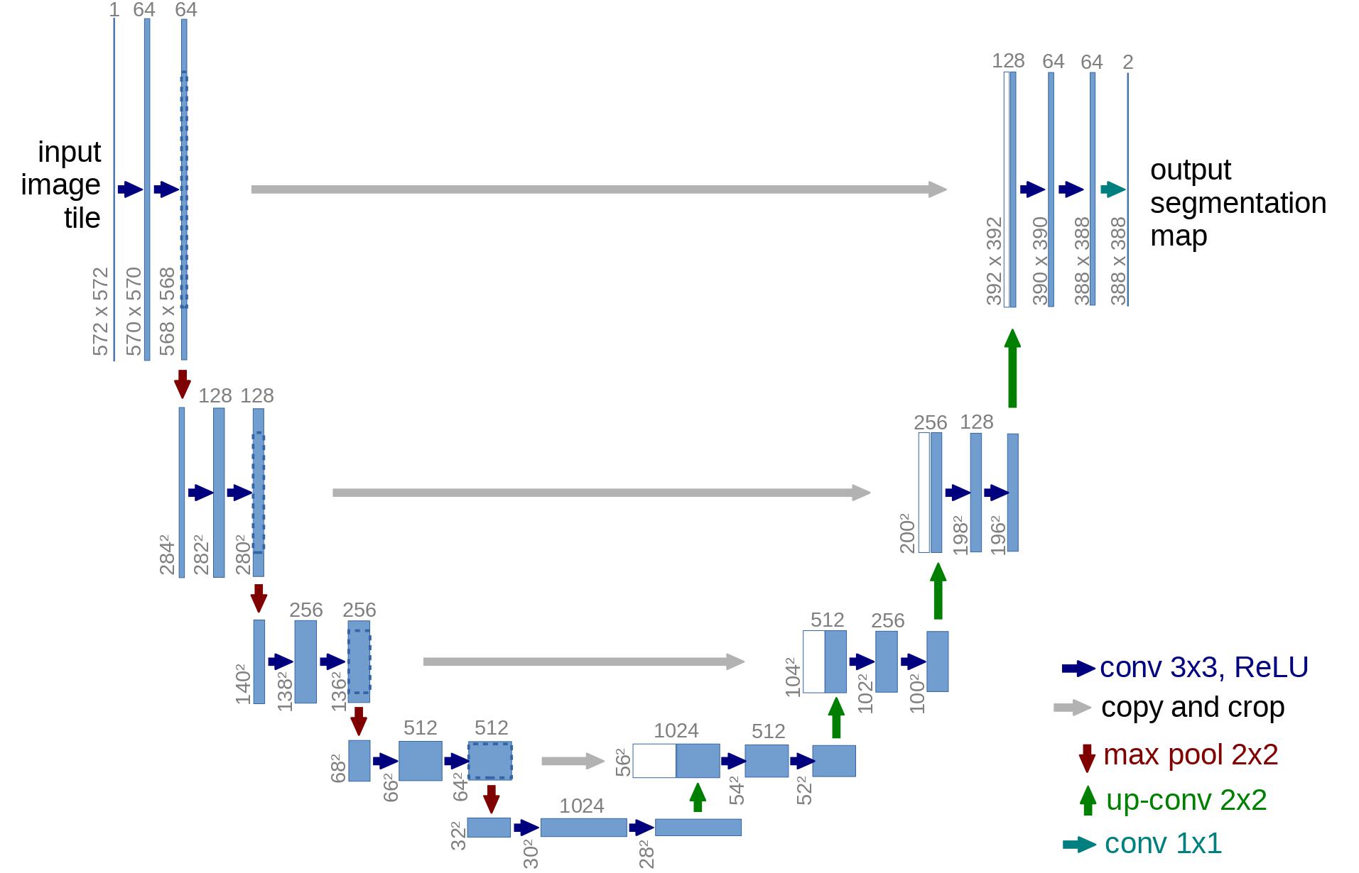
可以看出,U-Net 模型首先对输入进行下采样(即在空间分辨率方面使输入变小),然后执行上采样。
下面,我们将逐步实现这个网络。
网络辅助函数
首先,我们定义一些辅助函数和类,它们将在实现神经网络时使用。重要的是,我们定义了一个`Residual`模块,它简单地将输入添加到特定函数的输出中(换句话说,为特定函数添加了一个残差连接)。
我们还为上采样和下采样操作定义了别名。
def exists(x):
    return x is not None

def default(val, d):
    if exists(val):
        return val
    return d() if isfunction(d) else d


def num_to_groups(num, divisor):
    groups = num // divisor
    remainder = num % divisor
    arr = [divisor] * groups
    if remainder > 0:
        arr.append(remainder)
    return arr


class Residual(nn.Module):
    def __init__(self, fn):
        super().__init__()
        self.fn = fn

    def forward(self, x, *args, **kwargs):
        return self.fn(x, *args, **kwargs) + x


def Upsample(dim, dim_out=None):
    return nn.Sequential(
        nn.Upsample(scale_factor=2, mode="nearest"),
        nn.Conv2d(dim, default(dim_out, dim), 3, padding=1),
    )


def Downsample(dim, dim_out=None):
    # No More Strided Convolutions or Pooling
    return nn.Sequential(
        Rearrange("b c (h p1) (w p2) -> b (c p1 p2) h w", p1=2, p2=2),
        nn.Conv2d(dim * 4, default(dim_out, dim), 1),
    )
位置嵌入
由于神经网络的参数在时间(噪声水平)上是共享的,因此作者采用正弦位置嵌入来编码,这受到了Transformer(Vaswani et al., 2017)的启发。这使得神经网络“知道”它在批处理中的每个图像都在哪个特定时间步(噪声水平)下运行。
SinusoidalPositionEmbeddings模块将形状为`(batch_size, 1)`的张量作为输入(即批处理中几个嘈杂图像的噪声水平),并将其转换为形状为`(batch_size, dim)`的张量,其中`dim`是位置嵌入的维度。然后将其添加到每个残差块中,我们将在后面看到。
class SinusoidalPositionEmbeddings(nn.Module):
    def __init__(self, dim):
        super().__init__()
        self.dim = dim

    def forward(self, time):
        device = time.device
        half_dim = self.dim // 2
        embeddings = math.log(10000) / (half_dim - 1)
        embeddings = torch.exp(torch.arange(half_dim, device=device) * -embeddings)
        embeddings = time[:, None] * embeddings[None, :]
        embeddings = torch.cat((embeddings.sin(), embeddings.cos()), dim=-1)
        return embeddings
ResNet 块
接下来,我们定义 U-Net 模型的核心构建块。DDPM 作者采用了 Wide ResNet 块(Zagoruyko 等人,2016),但 Phil Wang 将标准卷积层替换为“权重标准化”版本,这与组归一化结合使用效果更好(详见(Kolesnikov 等人,2019))。
class WeightStandardizedConv2d(nn.Conv2d):
    """
    https://arxiv.org/abs/1903.10520
    weight standardization purportedly works synergistically with group normalization
    """

    def forward(self, x):
        eps = 1e-5 if x.dtype == torch.float32 else 1e-3

        weight = self.weight
        mean = reduce(weight, "o ... -> o 1 1 1", "mean")
        var = reduce(weight, "o ... -> o 1 1 1", partial(torch.var, unbiased=False))
        normalized_weight = (weight - mean) * (var + eps).rsqrt()

        return F.conv2d(
            x,
            normalized_weight,
            self.bias,
            self.stride,
            self.padding,
            self.dilation,
            self.groups,
        )


class Block(nn.Module):
    def __init__(self, dim, dim_out, groups=8):
        super().__init__()
        self.proj = WeightStandardizedConv2d(dim, dim_out, 3, padding=1)
        self.norm = nn.GroupNorm(groups, dim_out)
        self.act = nn.SiLU()

    def forward(self, x, scale_shift=None):
        x = self.proj(x)
        x = self.norm(x)

        if exists(scale_shift):
            scale, shift = scale_shift
            x = x * (scale + 1) + shift

        x = self.act(x)
        return x


class ResnetBlock(nn.Module):
    """https://arxiv.org/abs/1512.03385"""

    def __init__(self, dim, dim_out, *, time_emb_dim=None, groups=8):
        super().__init__()
        self.mlp = (
            nn.Sequential(nn.SiLU(), nn.Linear(time_emb_dim, dim_out * 2))
            if exists(time_emb_dim)
            else None
        )

        self.block1 = Block(dim, dim_out, groups=groups)
        self.block2 = Block(dim_out, dim_out, groups=groups)
        self.res_conv = nn.Conv2d(dim, dim_out, 1) if dim != dim_out else nn.Identity()

    def forward(self, x, time_emb=None):
        scale_shift = None
        if exists(self.mlp) and exists(time_emb):
            time_emb = self.mlp(time_emb)
            time_emb = rearrange(time_emb, "b c -> b c 1 1")
            scale_shift = time_emb.chunk(2, dim=1)

        h = self.block1(x, scale_shift=scale_shift)
        h = self.block2(h)
        return h + self.res_conv(x)
注意力模块
接下来,我们定义注意力模块,DDPM 的作者将其添加在卷积块之间。注意力是著名的 Transformer 架构(Vaswani et al., 2017)的基本组成部分,该架构在 AI 的各个领域都取得了巨大成功,从自然语言处理和视觉到蛋白质折叠。Phil Wang 采用了两种注意力变体:一种是常规的多头自注意力(如 Transformer 中使用的),另一种是线性注意力变体(Shen et al., 2018),其时间和内存需求随序列长度线性缩放,而常规注意力是二次方缩放。
有关注意力机制的详细解释,请参阅 Jay Allamar 的精彩博客文章。
class Attention(nn.Module):
    def __init__(self, dim, heads=4, dim_head=32):
        super().__init__()
        self.scale = dim_head**-0.5
        self.heads = heads
        hidden_dim = dim_head * heads
        self.to_qkv = nn.Conv2d(dim, hidden_dim * 3, 1, bias=False)
        self.to_out = nn.Conv2d(hidden_dim, dim, 1)

    def forward(self, x):
        b, c, h, w = x.shape
        qkv = self.to_qkv(x).chunk(3, dim=1)
        q, k, v = map(
            lambda t: rearrange(t, "b (h c) x y -> b h c (x y)", h=self.heads), qkv
        )
        q = q * self.scale

        sim = einsum("b h d i, b h d j -> b h i j", q, k)
        sim = sim - sim.amax(dim=-1, keepdim=True).detach()
        attn = sim.softmax(dim=-1)

        out = einsum("b h i j, b h d j -> b h i d", attn, v)
        out = rearrange(out, "b h (x y) d -> b (h d) x y", x=h, y=w)
        return self.to_out(out)

class LinearAttention(nn.Module):
    def __init__(self, dim, heads=4, dim_head=32):
        super().__init__()
        self.scale = dim_head**-0.5
        self.heads = heads
        hidden_dim = dim_head * heads
        self.to_qkv = nn.Conv2d(dim, hidden_dim * 3, 1, bias=False)

        self.to_out = nn.Sequential(nn.Conv2d(hidden_dim, dim, 1),
                                    nn.GroupNorm(1, dim))

    def forward(self, x):
        b, c, h, w = x.shape
        qkv = self.to_qkv(x).chunk(3, dim=1)
        q, k, v = map(
            lambda t: rearrange(t, "b (h c) x y -> b h c (x y)", h=self.heads), qkv
        )

        q = q.softmax(dim=-2)
        k = k.softmax(dim=-1)

        q = q * self.scale
        context = torch.einsum("b h d n, b h e n -> b h d e", k, v)

        out = torch.einsum("b h d e, b h d n -> b h e n", context, q)
        out = rearrange(out, "b h c (x y) -> b (h c) x y", h=self.heads, x=h, y=w)
        return self.to_out(out)
组归一化
DDPM 的作者将 U-Net 的卷积层/注意力层与组归一化(Wu et al., 2018)交织在一起。下面,我们定义了一个 `PreNorm` 类,它将用于在注意力层之前应用组归一化,我们将在后面看到。请注意,关于在 Transformer 中是在注意力之前还是之后应用归一化,一直存在争议。
class PreNorm(nn.Module):
    def __init__(self, dim, fn):
        super().__init__()
        self.fn = fn
        self.norm = nn.GroupNorm(1, dim)

    def forward(self, x):
        x = self.norm(x)
        return self.fn(x)
条件 U-Net
现在我们已经定义了所有构建块(位置嵌入、ResNet 块、注意力和组归一化),是时候定义整个神经网络了。回想一下,网络的工作是接收一批带噪声的图像及其各自的噪声水平,并输出添加到输入中的噪声。更正式地说:
- 网络接收一批形状为`(batch_size, num_channels, height, width)`的噪声图像和一批形状为`(batch_size, 1)`的噪声水平作为输入,并返回形状为`(batch_size, num_channels, height, width)`的张量
网络构建如下:
- 首先,对一批带噪声的图像应用卷积层,并为噪声水平计算位置嵌入。
- 接下来,应用一系列下采样阶段。每个下采样阶段由2个ResNet块+组归一化+注意力+残差连接+一个下采样操作组成。
- 在网络的中间,再次应用ResNet块,并穿插注意力。
- 接下来,应用一系列上采样阶段。每个上采样阶段由2个ResNet块+组归一化+注意力+残差连接+一个上采样操作组成。
- 最后,应用一个ResNet块,然后是一个卷积层。
最终,神经网络就像乐高积木一样堆叠层(但理解它们的工作原理很重要)。
class Unet(nn.Module):
    def __init__(
        self,
        dim,
        init_dim=None,
        out_dim=None,
        dim_mults=(1, 2, 4, 8),
        channels=3,
        self_condition=False,
        resnet_block_groups=4,
    ):
        super().__init__()

        # determine dimensions
        self.channels = channels
        self.self_condition = self_condition
        input_channels = channels * (2 if self_condition else 1)

        init_dim = default(init_dim, dim)
        self.init_conv = nn.Conv2d(input_channels, init_dim, 1, padding=0) # changed to 1 and 0 from 7,3

        dims = [init_dim, *map(lambda m: dim * m, dim_mults)]
        in_out = list(zip(dims[:-1], dims[1:]))

        block_klass = partial(ResnetBlock, groups=resnet_block_groups)

        # time embeddings
        time_dim = dim * 4

        self.time_mlp = nn.Sequential(
            SinusoidalPositionEmbeddings(dim),
            nn.Linear(dim, time_dim),
            nn.GELU(),
            nn.Linear(time_dim, time_dim),
        )

        # layers
        self.downs = nn.ModuleList([])
        self.ups = nn.ModuleList([])
        num_resolutions = len(in_out)

        for ind, (dim_in, dim_out) in enumerate(in_out):
            is_last = ind >= (num_resolutions - 1)

            self.downs.append(
                nn.ModuleList(
                    [
                        block_klass(dim_in, dim_in, time_emb_dim=time_dim),
                        block_klass(dim_in, dim_in, time_emb_dim=time_dim),
                        Residual(PreNorm(dim_in, LinearAttention(dim_in))),
                        Downsample(dim_in, dim_out)
                        if not is_last
                        else nn.Conv2d(dim_in, dim_out, 3, padding=1),
                    ]
                )
            )

        mid_dim = dims[-1]
        self.mid_block1 = block_klass(mid_dim, mid_dim, time_emb_dim=time_dim)
        self.mid_attn = Residual(PreNorm(mid_dim, Attention(mid_dim)))
        self.mid_block2 = block_klass(mid_dim, mid_dim, time_emb_dim=time_dim)

        for ind, (dim_in, dim_out) in enumerate(reversed(in_out)):
            is_last = ind == (len(in_out) - 1)

            self.ups.append(
                nn.ModuleList(
                    [
                        block_klass(dim_out + dim_in, dim_out, time_emb_dim=time_dim),
                        block_klass(dim_out + dim_in, dim_out, time_emb_dim=time_dim),
                        Residual(PreNorm(dim_out, LinearAttention(dim_out))),
                        Upsample(dim_out, dim_in)
                        if not is_last
                        else nn.Conv2d(dim_out, dim_in, 3, padding=1),
                    ]
                )
            )

        self.out_dim = default(out_dim, channels)

        self.final_res_block = block_klass(dim * 2, dim, time_emb_dim=time_dim)
        self.final_conv = nn.Conv2d(dim, self.out_dim, 1)

    def forward(self, x, time, x_self_cond=None):
        if self.self_condition:
            x_self_cond = default(x_self_cond, lambda: torch.zeros_like(x))
            x = torch.cat((x_self_cond, x), dim=1)

        x = self.init_conv(x)
        r = x.clone()

        t = self.time_mlp(time)

        h = []

        for block1, block2, attn, downsample in self.downs:
            x = block1(x, t)
            h.append(x)

            x = block2(x, t)
            x = attn(x)
            h.append(x)

            x = downsample(x)

        x = self.mid_block1(x, t)
        x = self.mid_attn(x)
        x = self.mid_block2(x, t)

        for block1, block2, attn, upsample in self.ups:
            x = torch.cat((x, h.pop()), dim=1)
            x = block1(x, t)

            x = torch.cat((x, h.pop()), dim=1)
            x = block2(x, t)
            x = attn(x)

            x = upsample(x)

        x = torch.cat((x, r), dim=1)

        x = self.final_res_block(x, t)
        return self.final_conv(x)
定义正向扩散过程
正向扩散过程在多个时间步中逐渐向真实分布中的图像添加噪声。这根据方差调度进行。最初的 DDPM 作者采用线性调度:
我们将正向过程方差设置为从线性增加到的常数。
然而,(Nichol et al., 2021) 的研究表明,采用余弦调度可以取得更好的结果。
下面,我们定义了时间步的各种调度(我们稍后会选择其中一个)。
def cosine_beta_schedule(timesteps, s=0.008):
    """
    cosine schedule as proposed in https://arxiv.org/abs/2102.09672
    """
    steps = timesteps + 1
    x = torch.linspace(0, timesteps, steps)
    alphas_cumprod = torch.cos(((x / timesteps) + s) / (1 + s) * torch.pi * 0.5) ** 2
    alphas_cumprod = alphas_cumprod / alphas_cumprod[0]
    betas = 1 - (alphas_cumprod[1:] / alphas_cumprod[:-1])
    return torch.clip(betas, 0.0001, 0.9999)

def linear_beta_schedule(timesteps):
    beta_start = 0.0001
    beta_end = 0.02
    return torch.linspace(beta_start, beta_end, timesteps)

def quadratic_beta_schedule(timesteps):
    beta_start = 0.0001
    beta_end = 0.02
    return torch.linspace(beta_start**0.5, beta_end**0.5, timesteps) ** 2

def sigmoid_beta_schedule(timesteps):
    beta_start = 0.0001
    beta_end = 0.02
    betas = torch.linspace(-6, 6, timesteps)
    return torch.sigmoid(betas) * (beta_end - beta_start) + beta_start
首先,让我们使用个时间步的线性调度,并定义我们将需要的来自的各种变量,例如方差的累积乘积。下面的每个变量都只是一个一维张量,存储从到的值。重要的是,我们还定义了一个`extract`函数,它允许我们为一批索引提取适当的索引。
timesteps = 300

# define beta schedule
betas = linear_beta_schedule(timesteps=timesteps)

# define alphas
alphas = 1. - betas
alphas_cumprod = torch.cumprod(alphas, axis=0)
alphas_cumprod_prev = F.pad(alphas_cumprod[:-1], (1, 0), value=1.0)
sqrt_recip_alphas = torch.sqrt(1.0 / alphas)

# calculations for diffusion q(x_t | x_{t-1}) and others
sqrt_alphas_cumprod = torch.sqrt(alphas_cumprod)
sqrt_one_minus_alphas_cumprod = torch.sqrt(1. - alphas_cumprod)

# calculations for posterior q(x_{t-1} | x_t, x_0)
posterior_variance = betas * (1. - alphas_cumprod_prev) / (1. - alphas_cumprod)

def extract(a, t, x_shape):
    batch_size = t.shape[0]
    out = a.gather(-1, t.cpu())
    return out.reshape(batch_size, *((1,) * (len(x_shape) - 1))).to(t.device)
我们将用猫的图像来说明在扩散过程的每个时间步如何添加噪声。
from PIL import Image
import requests

url = 'http://images.cocodataset.org/val2017/000000039769.jpg'
image = Image.open(requests.get(url, stream=True).raw) # PIL image of shape HWC
image

噪声被添加到 PyTorch 张量中,而不是 Pillow 图像中。我们首先定义图像转换,允许我们从 PIL 图像转换为 PyTorch 张量(我们可以在其上添加噪声),反之亦然。
这些转换相当简单:我们首先将图像除以进行归一化(使它们在范围内),然后确保它们在范围内。根据 DDPM 论文:
我们假设图像数据由中的整数组成,并线性缩放到。这确保了神经网络逆向过程在从标准正态先验开始时,以一致缩放的输入进行操作。
from torchvision.transforms import Compose, ToTensor, Lambda, ToPILImage, CenterCrop, Resize

image_size = 128
transform = Compose([
    Resize(image_size),
    CenterCrop(image_size),
    ToTensor(), # turn into torch Tensor of shape CHW, divide by 255
    Lambda(lambda t: (t * 2) - 1),

])

x_start = transform(image).unsqueeze(0)
x_start.shape
Output:
----------------------------------------------------------------------------------------------------
torch.Size([1, 3, 128, 128])
我们还定义了反向转换,它接受一个包含范围内值的 PyTorch 张量,并将其转换回 PIL 图像
import numpy as np

reverse_transform = Compose([
     Lambda(lambda t: (t + 1) / 2),
     Lambda(lambda t: t.permute(1, 2, 0)), # CHW to HWC
     Lambda(lambda t: t * 255.),
     Lambda(lambda t: t.numpy().astype(np.uint8)),
     ToPILImage(),
])
让我们验证一下
reverse_transform(x_start.squeeze())

我们现在可以像论文中那样定义正向扩散过程:
# forward diffusion (using the nice property)
def q_sample(x_start, t, noise=None):
    if noise is None:
        noise = torch.randn_like(x_start)

    sqrt_alphas_cumprod_t = extract(sqrt_alphas_cumprod, t, x_start.shape)
    sqrt_one_minus_alphas_cumprod_t = extract(
        sqrt_one_minus_alphas_cumprod, t, x_start.shape
    )

    return sqrt_alphas_cumprod_t * x_start + sqrt_one_minus_alphas_cumprod_t * noise
让我们在一个特定的时间步上测试它。
def get_noisy_image(x_start, t):
  # add noise
  x_noisy = q_sample(x_start, t=t)

  # turn back into PIL image
  noisy_image = reverse_transform(x_noisy.squeeze())

  return noisy_image
# take time step
t = torch.tensor([40])

get_noisy_image(x_start, t)
让我们在不同的时间步可视化这一点。
import matplotlib.pyplot as plt

# use seed for reproducability
torch.manual_seed(0)

# source: https://pytorch.ac.cn/vision/stable/auto_examples/plot_transforms.html#sphx-glr-auto-examples-plot-transforms-py
def plot(imgs, with_orig=False, row_title=None, **imshow_kwargs):
    if not isinstance(imgs[0], list):
        # Make a 2d grid even if there's just 1 row
        imgs = [imgs]

    num_rows = len(imgs)
    num_cols = len(imgs[0]) + with_orig
    fig, axs = plt.subplots(figsize=(200,200), nrows=num_rows, ncols=num_cols, squeeze=False)
    for row_idx, row in enumerate(imgs):
        row = [image] + row if with_orig else row
        for col_idx, img in enumerate(row):
            ax = axs[row_idx, col_idx]
            ax.imshow(np.asarray(img), **imshow_kwargs)
            ax.set(xticklabels=[], yticklabels=[], xticks=[], yticks=[])

    if with_orig:
        axs[0, 0].set(title='Original image')
        axs[0, 0].title.set_size(8)
    if row_title is not None:
        for row_idx in range(num_rows):
            axs[row_idx, 0].set(ylabel=row_title[row_idx])

    plt.tight_layout()
plot([get_noisy_image(x_start, torch.tensor([t])) for t in [0, 50, 100, 150, 199]])
这意味着我们现在可以根据上面定义的模型定义损失函数:
def p_losses(denoise_model, x_start, t, noise=None, loss_type="l1"):
    if noise is None:
        noise = torch.randn_like(x_start)

    x_noisy = q_sample(x_start=x_start, t=t, noise=noise)
    predicted_noise = denoise_model(x_noisy, t)

    if loss_type == 'l1':
        loss = F.l1_loss(noise, predicted_noise)
    elif loss_type == 'l2':
        loss = F.mse_loss(noise, predicted_noise)
    elif loss_type == "huber":
        loss = F.smooth_l1_loss(noise, predicted_noise)
    else:
        raise NotImplementedError()

    return loss
`denoise_model`将是上面定义的 U-Net。我们将使用真实噪声和预测噪声之间的 Huber 损失。
定义 PyTorch 数据集 + DataLoader
这里我们定义一个普通的PyTorch 数据集。该数据集简单地由真实数据集(如 Fashion-MNIST、CIFAR-10 或 ImageNet)中的图像组成,并线性缩放到。
每个图像都被调整为相同的大小。值得注意的是,图像也会随机水平翻转。根据论文:
我们在 CIFAR10 训练期间使用了随机水平翻转;我们尝试了带翻转和不带翻转的训练,发现翻转略微改善了样本质量。
在这里,我们使用 🤗 Datasets 库,轻松地从中心加载 Fashion MNIST 数据集。该数据集包含已经具有相同分辨率(即 28x28)的图像。
from datasets import load_dataset

# load dataset from the hub
dataset = load_dataset("fashion_mnist")
image_size = 28
channels = 1
batch_size = 128
接下来,我们定义一个函数,该函数将实时应用于整个数据集。我们为此使用了 `with_transform` 功能。该函数只应用了一些基本的图像预处理:随机水平翻转、重新缩放,最后使它们的值在范围内。
from torchvision import transforms
from torch.utils.data import DataLoader

# define image transformations (e.g. using torchvision)
transform = Compose([
            transforms.RandomHorizontalFlip(),
            transforms.ToTensor(),
            transforms.Lambda(lambda t: (t * 2) - 1)
])

# define function
def transforms(examples):
   examples["pixel_values"] = [transform(image.convert("L")) for image in examples["image"]]
   del examples["image"]

   return examples

transformed_dataset = dataset.with_transform(transforms).remove_columns("label")

# create dataloader
dataloader = DataLoader(transformed_dataset["train"], batch_size=batch_size, shuffle=True)
batch = next(iter(dataloader))
print(batch.keys())
Output:
----------------------------------------------------------------------------------------------------
dict_keys(['pixel_values'])
采样
由于我们将在训练期间从模型中采样(以跟踪进度),因此我们在下面定义了相应的代码。论文中将采样总结为算法2
从扩散模型生成新图像是通过逆转扩散过程来实现的:我们从开始,从高斯分布中采样纯噪声,然后使用我们的神经网络逐渐对其进行去噪(使用它学到的条件概率),直到我们到达时间步。如上所示,我们可以通过插入均值的重参数化,使用我们的噪声预测器,推导出稍微不那么去噪的图像。请记住,方差是提前已知的。
理想情况下,我们最终得到的图像看起来像是来自真实数据分布的。
下面的代码实现了这一点。
@torch.no_grad()
def p_sample(model, x, t, t_index):
    betas_t = extract(betas, t, x.shape)
    sqrt_one_minus_alphas_cumprod_t = extract(
        sqrt_one_minus_alphas_cumprod, t, x.shape
    )
    sqrt_recip_alphas_t = extract(sqrt_recip_alphas, t, x.shape)

    # Equation 11 in the paper
    # Use our model (noise predictor) to predict the mean
    model_mean = sqrt_recip_alphas_t * (
        x - betas_t * model(x, t) / sqrt_one_minus_alphas_cumprod_t
    )

    if t_index == 0:
        return model_mean
    else:
        posterior_variance_t = extract(posterior_variance, t, x.shape)
        noise = torch.randn_like(x)
        # Algorithm 2 line 4:
        return model_mean + torch.sqrt(posterior_variance_t) * noise

# Algorithm 2 (including returning all images)
@torch.no_grad()
def p_sample_loop(model, shape):
    device = next(model.parameters()).device

    b = shape[0]
    # start from pure noise (for each example in the batch)
    img = torch.randn(shape, device=device)
    imgs = []

    for i in tqdm(reversed(range(0, timesteps)), desc='sampling loop time step', total=timesteps):
        img = p_sample(model, img, torch.full((b,), i, device=device, dtype=torch.long), i)
        imgs.append(img.cpu().numpy())
    return imgs

@torch.no_grad()
def sample(model, image_size, batch_size=16, channels=3):
    return p_sample_loop(model, shape=(batch_size, channels, image_size, image_size))
请注意,上面的代码是原始实现的简化版本。我们发现我们的简化(与论文中的算法2一致)与原始、更复杂的实现一样有效,后者采用了裁剪。
训练模型
接下来,我们以常规 PyTorch 方式训练模型。我们还定义了一些逻辑,用于使用上面定义的 `sample` 方法定期保存生成的图像。
from pathlib import Path

def num_to_groups(num, divisor):
    groups = num // divisor
    remainder = num % divisor
    arr = [divisor] * groups
    if remainder > 0:
        arr.append(remainder)
    return arr

results_folder = Path("./results")
results_folder.mkdir(exist_ok = True)
save_and_sample_every = 1000
下面,我们定义模型,并将其移动到 GPU。我们还定义了一个标准优化器(Adam)。
from torch.optim import Adam

device = "cuda" if torch.cuda.is_available() else "cpu"

model = Unet(
    dim=image_size,
    channels=channels,
    dim_mults=(1, 2, 4,)
)
model.to(device)

optimizer = Adam(model.parameters(), lr=1e-3)
我们开始训练吧!
from torchvision.utils import save_image

epochs = 6

for epoch in range(epochs):
    for step, batch in enumerate(dataloader):
      optimizer.zero_grad()

      batch_size = batch["pixel_values"].shape[0]
      batch = batch["pixel_values"].to(device)

      # Algorithm 1 line 3: sample t uniformally for every example in the batch
      t = torch.randint(0, timesteps, (batch_size,), device=device).long()

      loss = p_losses(model, batch, t, loss_type="huber")

      if step % 100 == 0:
        print("Loss:", loss.item())

      loss.backward()
      optimizer.step()

      # save generated images
      if step != 0 and step % save_and_sample_every == 0:
        milestone = step // save_and_sample_every
        batches = num_to_groups(4, batch_size)
        all_images_list = list(map(lambda n: sample(model, batch_size=n, channels=channels), batches))
        all_images = torch.cat(all_images_list, dim=0)
        all_images = (all_images + 1) * 0.5
        save_image(all_images, str(results_folder / f'sample-{milestone}.png'), nrow = 6)
Output:
----------------------------------------------------------------------------------------------------
Loss: 0.46477368474006653
Loss: 0.12143351882696152
Loss: 0.08106148988008499
Loss: 0.0801810547709465
Loss: 0.06122320517897606
Loss: 0.06310459971427917
Loss: 0.05681884288787842
Loss: 0.05729678273200989
Loss: 0.05497899278998375
Loss: 0.04439849033951759
Loss: 0.05415581166744232
Loss: 0.06020551547408104
Loss: 0.046830907464027405
Loss: 0.051029372960329056
Loss: 0.0478244312107563
Loss: 0.046767622232437134
Loss: 0.04305662214756012
Loss: 0.05216279625892639
Loss: 0.04748568311333656
Loss: 0.05107741802930832
Loss: 0.04588869959115982
Loss: 0.043014321476221085
Loss: 0.046371955424547195
Loss: 0.04952816292643547
Loss: 0.04472338408231735
采样(推理)
要从模型中采样,我们可以直接使用上面定义的采样函数
# sample 64 images
samples = sample(model, image_size=image_size, batch_size=64, channels=channels)

# show a random one
random_index = 5
plt.imshow(samples[-1][random_index].reshape(image_size, image_size, channels), cmap="gray")
看起来模型能够生成一件漂亮的 T 恤!请记住,我们训练的数据集分辨率相当低 (28x28)。
我们还可以创建去噪过程的 GIF
import matplotlib.animation as animation

random_index = 53

fig = plt.figure()
ims = []
for i in range(timesteps):
    im = plt.imshow(samples[i][random_index].reshape(image_size, image_size, channels), cmap="gray", animated=True)
    ims.append([im])

animate = animation.ArtistAnimation(fig, ims, interval=50, blit=True, repeat_delay=1000)
animate.save('diffusion.gif')
plt.show()

后续阅读
请注意,DDPM 论文表明扩散模型是(无)条件图像生成的一个有前途的方向。此后,这一领域(极大地)得到了改进,尤其是在文本条件图像生成方面。下面,我们列出了一些重要的(但远非详尽的)后续工作
- 改进的去噪扩散概率模型 (Nichol 等人,2021):发现学习条件分布的方差(除了均值)有助于提高性能
- 用于高保真图像生成的级联扩散模型 (Ho 等人,2021):引入了级联扩散,它包含多个扩散模型的管道,这些模型生成分辨率不断提高的图像,用于高保真图像合成
- 扩散模型在图像合成方面击败 GANs (Dhariwal 等人,2021):通过改进 U-Net 架构并引入分类器引导,表明扩散模型可以实现优于当前最先进生成模型的图像样本质量
- 无分类器扩散引导 (Ho 等人,2021):通过使用单个神经网络联合训练条件和无条件扩散模型,表明您不需要分类器来引导扩散模型
- 使用 CLIP 潜在变量进行分层文本条件图像生成 (DALL-E 2) (Ramesh 等人,2022):使用先验将文本描述转换为 CLIP 图像嵌入,然后扩散模型将其解码为图像
- 具有深度语言理解的光逼真文本到图像扩散模型 (ImageGen) (Saharia 等人,2022):表明将大型预训练语言模型(例如 T5)与级联扩散相结合在文本到图像合成方面效果很好
请注意,此列表仅包含截至撰写本文时(2022 年 6 月 7 日)的重要作品。
目前,扩散模型的主要(也许是唯一)缺点似乎是它们需要多次前向传播才能生成图像(GANs 等生成模型则不需要)。然而,正在进行的研究正在实现仅在 10 个去噪步骤中进行高保真生成。