开源 AI 食谱文档
在自定义数据集上微调目标检测模型🖼,在Spaces上部署,以及Gradio API集成
并获得增强的文档体验
开始使用
在自定义数据集上微调目标检测模型🖼,在Spaces上部署,以及Gradio API集成
作者: Sergio Paniego
在本Notebook中,我们将使用自定义数据集微调一个目标检测模型——具体来说是DETR。我们将利用Hugging Face生态系统来完成此任务。
我们的方法涉及从预训练的DETR模型开始,并在一个自定义的时尚图像标注数据集Fashionpedia上进行微调。通过这样做,我们将使模型更好地识别和检测时尚领域内的物体。
成功微调模型后,我们将在Hugging Face上将其部署为Gradio Space。此外,我们还将探索如何使用Gradio API与部署的模型进行交互,从而实现与托管Space的无缝通信,并为实际应用开启新的可能性。

1. 安装依赖项
让我们首先安装微调目标检测模型所需的库。
!pip install -U -q datasets transformers[torch] timm wandb torchmetrics matplotlib albumentations
# Tested with datasets==2.21.0, transformers==4.44.2 timm==1.0.9, wandb==0.17.9 torchmetrics==1.4.1
2. 加载数据集📁
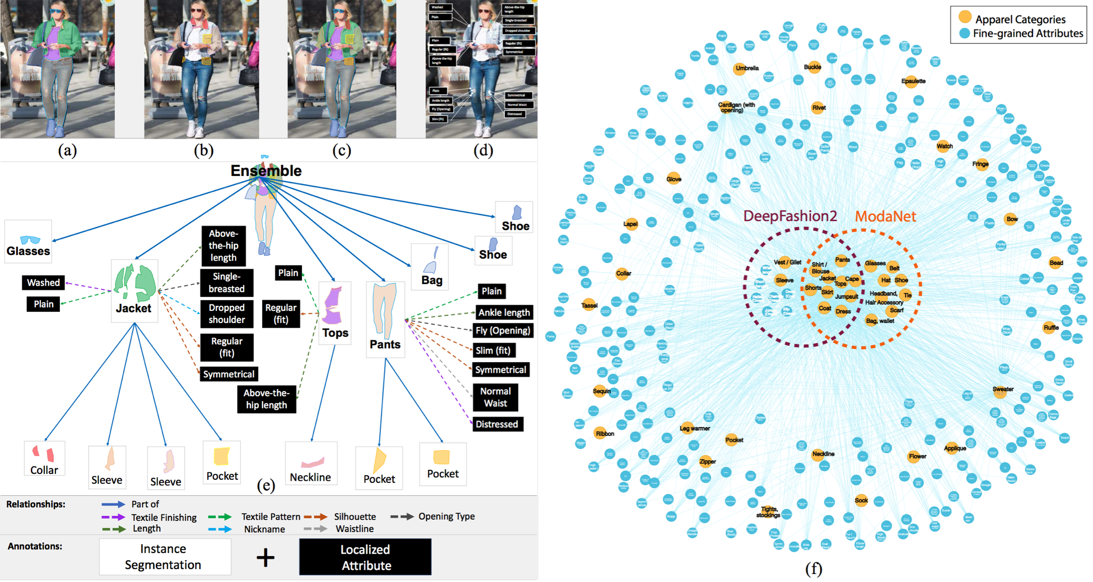
📁 我们将使用的数据集是Fashionpedia,它来自论文Fashionpedia: Ontology, Segmentation, and an Attribute Localization Dataset。作者将其描述为:
Fashionpedia is a dataset which consists of two parts: (1) an ontology built by fashion experts containing 27 main apparel categories, 19 apparel parts, 294 fine-grained attributes and their relationships; (2) a dataset with 48k everyday and celebrity event fashion images annotated with segmentation masks and their associated per-mask fine-grained attributes, built upon the Fashionpedia ontology.数据集包括:
- 46,781张图片 🖼
- 342,182个边界框 📦
它在Hugging Face上可用:Fashionpedia数据集
from datasets import load_dataset

dataset = load_dataset("detection-datasets/fashionpedia")dataset
查看其中一个内部结构的示例
dataset["train"][0]3. 获取数据集的训练和测试拆分➗
数据集包含两个拆分:训练和测试。我们将使用训练拆分来微调模型,并使用测试拆分进行验证。
train_dataset = dataset["train"]
test_dataset = dataset["val"]
可选
在下一个注释单元格中,我们随机抽取原始数据集的1%作为训练和测试拆分。这种方法用于加速训练过程,因为数据集包含大量示例。
为获得最佳结果,我们建议跳过这两个单元格并使用完整数据集。但是,如果需要,您可以取消注释它们。
"""
def create_sample(dataset, sample_fraction=0.01, seed=42):
    sample_size = int(sample_fraction * len(dataset))
    sampled_dataset = dataset.shuffle(seed=seed).select(range(sample_size))
    print(f"Original size: {len(dataset)}")
    print(f"Sample size: {len(sampled_dataset)}")
    return sampled_dataset

# Apply function to both splits
train_dataset = create_sample(train_dataset)
test_dataset = create_sample(test_dataset)
"""
4. 可视化数据集中包含其对象的一个示例👀
现在我们已经加载了数据集,让我们可视化一个示例及其标注对象。
生成id2label和label2id
这些变量包含对象ID与其对应标签之间的映射。`id2label`从ID映射到标签,而`label2id`从标签映射到ID。
import numpy as np
from PIL import Image, ImageDraw


id2label = {
    0: "shirt, blouse",
    1: "top, t-shirt, sweatshirt",
    2: "sweater",
    3: "cardigan",
    4: "jacket",
    5: "vest",
    6: "pants",
    7: "shorts",
    8: "skirt",
    9: "coat",
    10: "dress",
    11: "jumpsuit",
    12: "cape",
    13: "glasses",
    14: "hat",
    15: "headband, head covering, hair accessory",
    16: "tie",
    17: "glove",
    18: "watch",
    19: "belt",
    20: "leg warmer",
    21: "tights, stockings",
    22: "sock",
    23: "shoe",
    24: "bag, wallet",
    25: "scarf",
    26: "umbrella",
    27: "hood",
    28: "collar",
    29: "lapel",
    30: "epaulette",
    31: "sleeve",
    32: "pocket",
    33: "neckline",
    34: "buckle",
    35: "zipper",
    36: "applique",
    37: "bead",
    38: "bow",
    39: "flower",
    40: "fringe",
    41: "ribbon",
    42: "rivet",
    43: "ruffle",
    44: "sequin",
    45: "tassel",
}


label2id = {v: k for k, v in id2label.items()}
让我们绘制一张图片!🎨
现在,让我们可视化数据集中的一张图片,以更好地了解它的外观。
>>> def draw_image_from_idx(dataset, idx):
...     sample = dataset[idx]
...     image = sample["image"]
...     annotations = sample["objects"]
...     draw = ImageDraw.Draw(image)
...     width, height = sample["width"], sample["height"]

...     print(annotations)

...     for i in range(len(annotations["bbox_id"])):
...         box = annotations["bbox"][i]
...         x1, y1, x2, y2 = tuple(box)
...         draw.rectangle((x1, y1, x2, y2), outline="red", width=3)
...         draw.text((x1, y1), id2label[annotations["category"][i]], fill="green")

...     return image


>>> draw_image_from_idx(dataset=train_dataset, idx=10)  # You can test changing this id
{'bbox_id': [158977, 158978, 158979, 158980, 158981, 158982, 158983], 'category': [1, 23, 23, 6, 31, 31, 33], 'bbox': [[210.0, 225.0, 536.0, 784.0], [290.0, 897.0, 350.0, 1015.0], [464.0, 950.0, 534.0, 1021.0], [313.0, 407.0, 524.0, 954.0], [268.0, 229.0, 333.0, 563.0], [489.0, 247.0, 528.0, 591.0], [387.0, 225.0, 450.0, 253.0]], 'area': [69960, 2449, 1788, 75418, 15149, 5998, 479]}
让我们再可视化一些图片📸
现在,让我们看看数据集中的更多图片,以获得更广泛的数据视图。
>>> import matplotlib.pyplot as plt


>>> def plot_images(dataset, indices):
...     """
...     Plot images and their annotations.
...     """
...     num_cols = 3
...     num_rows = int(np.ceil(len(indices) / num_cols))
...     fig, axes = plt.subplots(num_rows, num_cols, figsize=(15, 10))

...     for i, idx in enumerate(indices):
...         row = i // num_cols
...         col = i % num_cols

...         image = draw_image_from_idx(dataset, idx)

...         axes[row, col].imshow(image)
...         axes[row, col].axis("off")

...     for j in range(i + 1, num_rows * num_cols):
...         fig.delaxes(axes.flatten()[j])

...     plt.tight_layout()
...     plt.show()


>>> plot_images(train_dataset, range(9))
{'bbox_id': [150311, 150312, 150313, 150314], 'category': [23, 23, 33, 10], 'bbox': [[445.0, 910.0, 505.0, 983.0], [239.0, 940.0, 284.0, 994.0], [298.0, 282.0, 386.0, 352.0], [210.0, 282.0, 448.0, 665.0]], 'area': [1422, 843, 373, 56375]} {'bbox_id': [158953, 158954, 158955, 158956, 158957, 158958, 158959, 158960, 158961, 158962], 'category': [2, 33, 31, 31, 13, 7, 22, 22, 23, 23], 'bbox': [[182.0, 220.0, 472.0, 647.0], [294.0, 221.0, 407.0, 257.0], [405.0, 297.0, 472.0, 647.0], [182.0, 264.0, 266.0, 621.0], [284.0, 135.0, 372.0, 169.0], [238.0, 537.0, 414.0, 606.0], [351.0, 732.0, 417.0, 922.0], [202.0, 749.0, 270.0, 930.0], [200.0, 921.0, 256.0, 979.0], [373.0, 903.0, 455.0, 966.0]], 'area': [87267, 1220, 16895, 18541, 1468, 9360, 8629, 8270, 2717, 3121]} {'bbox_id': [169196, 169197, 169198, 169199, 169200, 169201, 169202, 169203, 169204, 169205, 169206, 169207, 169208, 169209, 169210], 'category': [13, 29, 28, 32, 32, 31, 31, 0, 31, 31, 18, 4, 6, 23, 23], 'bbox': [[441.0, 132.0, 499.0, 150.0], [412.0, 164.0, 494.0, 295.0], [427.0, 164.0, 476.0, 207.0], [406.0, 326.0, 448.0, 335.0], [484.0, 327.0, 508.0, 334.0], [366.0, 323.0, 395.0, 372.0], [496.0, 271.0, 523.0, 302.0], [366.0, 164.0, 523.0, 372.0], [360.0, 186.0, 406.0, 332.0], [502.0, 201.0, 534.0, 321.0], [496.0, 259.0, 515.0, 278.0], [360.0, 164.0, 534.0, 411.0], [403.0, 384.0, 510.0, 638.0], [393.0, 584.0, 430.0, 663.0], [449.0, 638.0, 518.0, 681.0]], 'area': [587, 2922, 931, 262, 111, 1171, 540, 3981, 4457, 1724, 188, 26621, 16954, 2167, 1773]} {'bbox_id': [167967, 167968, 167969, 167970, 167971, 167972, 167973, 167974, 167975, 167976, 167977, 167978, 167979, 167980, 167981, 167982, 167983, 167984, 167985, 167986, 167987, 167988, 167989, 167990, 167991, 167992, 167993, 167994, 167995, 167996, 167997, 167998, 167999, 168000, 168001, 168002, 168003, 168004, 168005, 168006, 168007, 168008, 168009, 168010, 168011, 168012, 168013, 168014, 168015, 168016, 168017, 168018, 168019, 168020, 168021, 168022, 168023, 168024, 168025, 168026, 168027, 168028, 168029, 168030, 168031, 168032, 168033, 168034, 168035, 168036, 168037, 168038, 168039, 168040], 'category': [6, 23, 23, 31, 31, 4, 1, 35, 32, 35, 35, 35, 35, 28, 35, 42, 42, 42, 42, 42, 42, 42, 42, 42, 42, 42, 42, 42, 42, 42, 42, 42, 42, 42, 42, 42, 42, 42, 42, 42, 42, 42, 42, 42, 42, 42, 42, 42, 42, 42, 42, 42, 42, 42, 42, 42, 42, 42, 42, 42, 42, 42, 42, 42, 42, 42, 42, 42, 42, 42, 42, 42, 42, 33], 'bbox': [[300.0, 421.0, 460.0, 846.0], [383.0, 841.0, 432.0, 899.0], [304.0, 740.0, 347.0, 831.0], [246.0, 222.0, 295.0, 505.0], [456.0, 229.0, 492.0, 517.0], [246.0, 169.0, 492.0, 517.0], [355.0, 213.0, 450.0, 433.0], [289.0, 353.0, 303.0, 427.0], [442.0, 288.0, 460.0, 340.0], [451.0, 290.0, 458.0, 304.0], [407.0, 238.0, 473.0, 486.0], [487.0, 501.0, 491.0, 517.0], [246.0, 455.0, 252.0, 505.0], [340.0, 169.0, 442.0, 238.0], [348.0, 230.0, 372.0, 476.0], [411.0, 179.0, 414.0, 182.0], [414.0, 183.0, 418.0, 186.0], [418.0, 187.0, 421.0, 190.0], [421.0, 192.0, 425.0, 195.0], [424.0, 196.0, 428.0, 199.0], [426.0, 200.0, 430.0, 204.0], [429.0, 204.0, 433.0, 208.0], [431.0, 209.0, 435.0, 213.0], [433.0, 214.0, 437.0, 218.0], [434.0, 218.0, 438.0, 222.0], [436.0, 223.0, 440.0, 226.0], [437.0, 227.0, 441.0, 231.0], [438.0, 232.0, 442.0, 235.0], [433.0, 232.0, 437.0, 236.0], [429.0, 233.0, 432.0, 237.0], [423.0, 233.0, 426.0, 237.0], [417.0, 233.0, 421.0, 237.0], [353.0, 172.0, 355.0, 174.0], [353.0, 175.0, 354.0, 177.0], [351.0, 178.0, 353.0, 181.0], [350.0, 182.0, 351.0, 184.0], [347.0, 187.0, 350.0, 189.0], [346.0, 190.0, 349.0, 193.0], [345.0, 194.0, 348.0, 197.0], [344.0, 199.0, 347.0, 202.0], [342.0, 204.0, 346.0, 207.0], [342.0, 208.0, 345.0, 211.0], [342.0, 212.0, 344.0, 215.0], [342.0, 217.0, 345.0, 220.0], [344.0, 221.0, 346.0, 224.0], [348.0, 222.0, 350.0, 225.0], [353.0, 223.0, 356.0, 226.0], [359.0, 223.0, 361.0, 226.0], [364.0, 223.0, 366.0, 226.0], [247.0, 448.0, 253.0, 454.0], [251.0, 454.0, 254.0, 456.0], [252.0, 460.0, 255.0, 463.0], [252.0, 466.0, 255.0, 469.0], [253.0, 471.0, 255.0, 475.0], [253.0, 478.0, 255.0, 481.0], [253.0, 483.0, 256.0, 486.0], [254.0, 489.0, 256.0, 492.0], [254.0, 495.0, 256.0, 497.0], [247.0, 457.0, 249.0, 460.0], [247.0, 463.0, 249.0, 466.0], [248.0, 469.0, 249.0, 471.0], [248.0, 476.0, 250.0, 478.0], [248.0, 481.0, 250.0, 483.0], [249.0, 486.0, 250.0, 488.0], [487.0, 459.0, 490.0, 461.0], [487.0, 465.0, 490.0, 467.0], [487.0, 471.0, 490.0, 472.0], [487.0, 476.0, 489.0, 478.0], [486.0, 482.0, 489.0, 484.0], [486.0, 488.0, 489.0, 490.0], [486.0, 494.0, 488.0, 496.0], [486.0, 500.0, 488.0, 501.0], [485.0, 505.0, 487.0, 507.0], [365.0, 213.0, 409.0, 226.0]], 'area': [44062, 2140, 2633, 9206, 5905, 44791, 12948, 211, 335, 43, 691, 62, 104, 2169, 439, 9, 10, 9, 8, 9, 14, 10, 13, 13, 11, 11, 10, 10, 12, 10, 10, 14, 4, 2, 4, 2, 5, 6, 7, 7, 8, 7, 6, 7, 5, 5, 7, 6, 5, 12, 5, 7, 8, 6, 6, 6, 4, 4, 6, 5, 2, 4, 4, 2, 6, 6, 3, 4, 6, 6, 4, 2, 4, 94]} {'bbox_id': [168041, 168042, 168043, 168044, 168045, 168046, 168047], 'category': [10, 32, 35, 31, 4, 29, 33], 'bbox': [[238.0, 309.0, 471.0, 1022.0], [234.0, 572.0, 331.0, 602.0], [235.0, 580.0, 324.0, 599.0], [119.0, 318.0, 343.0, 856.0], [111.0, 262.0, 518.0, 1022.0], [166.0, 262.0, 393.0, 492.0], [238.0, 309.0, 278.0, 324.0]], 'area': [12132, 1548, 755, 43926, 178328, 9316, 136]} {'bbox_id': [160050, 160051, 160052, 160053, 160054, 160055], 'category': [10, 31, 31, 23, 23, 33], 'bbox': [[290.0, 364.0, 429.0, 665.0], [304.0, 369.0, 397.0, 508.0], [290.0, 468.0, 310.0, 522.0], [213.0, 842.0, 294.0, 905.0], [446.0, 840.0, 536.0, 896.0], [311.0, 364.0, 354.0, 379.0]], 'area': [26873, 5301, 747, 1438, 1677, 71]} {'bbox_id': [160056, 160057, 160058, 160059, 160060, 160061, 160062, 160063, 160064, 160065, 160066], 'category': [10, 36, 42, 42, 42, 42, 42, 42, 42, 23, 33], 'bbox': [[127.0, 198.0, 451.0, 949.0], [277.0, 336.0, 319.0, 402.0], [340.0, 343.0, 344.0, 347.0], [321.0, 338.0, 327.0, 343.0], [336.0, 361.0, 342.0, 365.0], [329.0, 321.0, 333.0, 326.0], [313.0, 294.0, 319.0, 300.0], [330.0, 299.0, 334.0, 304.0], [295.0, 330.0, 300.0, 334.0], [332.0, 926.0, 376.0, 946.0], [284.0, 198.0, 412.0, 270.0]], 'area': [137575, 1915, 14, 24, 18, 15, 25, 16, 16, 740, 586]} {'bbox_id': [158963, 158964, 158965, 158966, 158967, 158968, 158969, 158970, 158971], 'category': [1, 31, 31, 7, 22, 22, 23, 23, 33], 'bbox': [[262.0, 449.0, 435.0, 686.0], [399.0, 471.0, 435.0, 686.0], [262.0, 451.0, 294.0, 662.0], [276.0, 603.0, 423.0, 726.0], [291.0, 759.0, 343.0, 934.0], [341.0, 749.0, 401.0, 947.0], [302.0, 919.0, 337.0, 994.0], [323.0, 925.0, 374.0, 1005.0], [343.0, 456.0, 366.0, 467.0]], 'area': [22330, 4422, 4846, 14000, 6190, 6997, 1547, 2107, 49]} {'bbox_id': [158972, 158973, 158974, 158975, 158976], 'category': [23, 23, 28, 10, 5], 'bbox': [[412.0, 588.0, 451.0, 631.0], [333.0, 585.0, 357.0, 627.0], [361.0, 243.0, 396.0, 257.0], [303.0, 243.0, 447.0, 517.0], [330.0, 259.0, 425.0, 324.0]], 'area': [949, 737, 133, 17839, 2916]}
5. 过滤无效边界框❌
作为数据集预处理的第一步,我们将过滤掉一些无效的边界框。在审查数据集后,我们发现一些边界框没有有效的结构。因此,我们将丢弃这些无效条目。
>>> from datasets import Dataset


>>> def filter_invalid_bboxes(example):
...     valid_bboxes = []
...     valid_bbox_ids = []
...     valid_categories = []
...     valid_areas = []

...     for i, bbox in enumerate(example["objects"]["bbox"]):
...         x_min, y_min, x_max, y_max = bbox[:4]
...         if x_min < x_max and y_min < y_max:
...             valid_bboxes.append(bbox)
...             valid_bbox_ids.append(example["objects"]["bbox_id"][i])
...             valid_categories.append(example["objects"]["category"][i])
...             valid_areas.append(example["objects"]["area"][i])
...         else:
...             print(
...                 f"Image with invalid bbox: {example['image_id']} Invalid bbox detected and discarded: {bbox} - bbox_id: {example['objects']['bbox_id'][i]} - category: {example['objects']['category'][i]}"
...             )

...     example["objects"]["bbox"] = valid_bboxes
...     example["objects"]["bbox_id"] = valid_bbox_ids
...     example["objects"]["category"] = valid_categories
...     example["objects"]["area"] = valid_areas

...     return example


>>> train_dataset = train_dataset.map(filter_invalid_bboxes)
>>> test_dataset = test_dataset.map(filter_invalid_bboxes)
Image with invalid bbox: 8396 Invalid bbox detected and discarded: [0.0, 0.0, 0.0, 0.0] - bbox_id: 139952 - category: 42 Image with invalid bbox: 19725 Invalid bbox detected and discarded: [0.0, 0.0, 0.0, 0.0] - bbox_id: 23298 - category: 42 Image with invalid bbox: 19725 Invalid bbox detected and discarded: [0.0, 0.0, 0.0, 0.0] - bbox_id: 23299 - category: 42 Image with invalid bbox: 21696 Invalid bbox detected and discarded: [0.0, 0.0, 0.0, 0.0] - bbox_id: 277148 - category: 42 Image with invalid bbox: 23055 Invalid bbox detected and discarded: [0.0, 0.0, 0.0, 0.0] - bbox_id: 287029 - category: 33 Image with invalid bbox: 23671 Invalid bbox detected and discarded: [0.0, 0.0, 0.0, 0.0] - bbox_id: 290142 - category: 42 Image with invalid bbox: 26549 Invalid bbox detected and discarded: [0.0, 0.0, 0.0, 0.0] - bbox_id: 311943 - category: 37 Image with invalid bbox: 26834 Invalid bbox detected and discarded: [0.0, 0.0, 0.0, 0.0] - bbox_id: 309141 - category: 37 Image with invalid bbox: 31748 Invalid bbox detected and discarded: [0.0, 0.0, 0.0, 0.0] - bbox_id: 262063 - category: 42 Image with invalid bbox: 34253 Invalid bbox detected and discarded: [0.0, 0.0, 0.0, 0.0] - bbox_id: 315750 - category: 19
>>> print(train_dataset)
>>> print(test_dataset)
Dataset({
features: ['image_id', 'image', 'width', 'height', 'objects'],
num_rows: 45623
})
Dataset({
features: ['image_id', 'image', 'width', 'height', 'objects'],
num_rows: 1158
})
6. 可视化类别出现次数👀
让我们通过绘制每个类别的出现次数来进一步探索数据集。这将帮助我们了解类别的分布并识别任何潜在的偏差。
id_list = []
category_examples = {}
for example in train_dataset:
    id_list += example["objects"]["bbox_id"]
    for category in example["objects"]["category"]:
        if id2label[category] not in category_examples:
            category_examples[id2label[category]] = 1
        else:
            category_examples[id2label[category]] += 1

id_list.sort()>>> import matplotlib.pyplot as plt
>>> categories = list(category_examples.keys())
>>> values = list(category_examples.values())
>>> fig, ax = plt.subplots(figsize=(12, 8))
>>> bars = ax.bar(categories, values, color="skyblue")
>>> ax.set_xlabel("Categories", fontsize=14)
>>> ax.set_ylabel("Number of Occurrences", fontsize=14)
>>> ax.set_title("Number of Occurrences by Category", fontsize=16)
>>> ax.set_xticklabels(categories, rotation=90, ha="right")
>>> ax.grid(axis="y", linestyle="--", alpha=0.7)
>>> for bar in bars:
... height = bar.get_height()
... ax.text(bar.get_x() + bar.get_width() / 2.0, height, f"{height}", ha="center", va="bottom", fontsize=10)
>>> plt.tight_layout()
>>> plt.show()
我们可以观察到,某些类别,例如“鞋子”或“袖子”,在数据集中出现次数过多。这表明数据集可能存在不平衡,某些类别比其他类别更频繁地出现。识别这些不平衡对于解决模型训练中潜在的偏差至关重要。
7. 向数据集中添加数据增强
数据增强🪄 对于提高目标检测任务的性能至关重要。在本节中,我们将利用Albumentations的功能来有效增强我们的数据集。
Albumentations提供了一系列针对目标检测的强大增强技术。它允许进行各种转换,同时确保准确调整边界框。这些功能有助于生成更多样化的数据集,提高模型的鲁棒性和泛化能力。
import albumentations as A

train_transform = A.Compose(
    [
        A.LongestMaxSize(500),
        A.PadIfNeeded(500, 500, border_mode=0, value=(0, 0, 0)),
        A.HorizontalFlip(p=0.5),
        A.RandomBrightnessContrast(p=0.5),
        A.HueSaturationValue(p=0.5),
        A.Rotate(limit=10, p=0.5),
        A.RandomScale(scale_limit=0.2, p=0.5),
        A.GaussianBlur(p=0.5),
        A.GaussNoise(p=0.5),
    ],
    bbox_params=A.BboxParams(format="pascal_voc", label_fields=["category"]),
)

val_transform = A.Compose(
    [
        A.LongestMaxSize(500),
        A.PadIfNeeded(500, 500, border_mode=0, value=(0, 0, 0)),
    ],
    bbox_params=A.BboxParams(format="pascal_voc", label_fields=["category"]),
)
8. 从模型检查点初始化图像处理器🎆
我们将使用预训练的模型检查点实例化图像处理器。在这种情况下,我们使用的是facebook/detr-resnet-50-dc5模型。
from transformers import AutoImageProcessor

checkpoint = "facebook/detr-resnet-50-dc5"
image_processor = AutoImageProcessor.from_pretrained(checkpoint)
添加处理数据集的方法
我们现在将添加处理数据集的方法。这些方法将处理图像和标注的转换等任务,以确保它们与模型兼容。
def formatted_anns(image_id, category, area, bbox):
    annotations = []
    for i in range(0, len(category)):
        new_ann = {
            "image_id": image_id,
            "category_id": category[i],
            "isCrowd": 0,
            "area": area[i],
            "bbox": list(bbox[i]),
        }
        annotations.append(new_ann)

    return annotations


def convert_voc_to_coco(bbox):
    xmin, ymin, xmax, ymax = bbox
    width = xmax - xmin
    height = ymax - ymin
    return [xmin, ymin, width, height]


def transform_aug_ann(examples, transform):
    image_ids = examples["image_id"]
    images, bboxes, area, categories = [], [], [], []
    for image, objects in zip(examples["image"], examples["objects"]):
        image = np.array(image.convert("RGB"))[:, :, ::-1]
        out = transform(image=image, bboxes=objects["bbox"], category=objects["category"])

        area.append(objects["area"])
        images.append(out["image"])

        # Convert to COCO format
        converted_bboxes = [convert_voc_to_coco(bbox) for bbox in out["bboxes"]]
        bboxes.append(converted_bboxes)

        categories.append(out["category"])

    targets = [
        {"image_id": id_, "annotations": formatted_anns(id_, cat_, ar_, box_)}
        for id_, cat_, ar_, box_ in zip(image_ids, categories, area, bboxes)
    ]

    return image_processor(images=images, annotations=targets, return_tensors="pt")


def transform_train(examples):
    return transform_aug_ann(examples, transform=train_transform)


def transform_val(examples):
    return transform_aug_ann(examples, transform=val_transform)


train_dataset_transformed = train_dataset.with_transform(transform_train)
test_dataset_transformed = test_dataset.with_transform(transform_val)
9. 绘制增强示例🎆
我们即将进入模型训练阶段!在此之前,让我们可视化一些增强后的样本。这将使我们能够再次检查增强是否适合且有效地用于训练过程。
>>> # Updated draw function to accept an optional transform
>>> def draw_augmented_image_from_idx(dataset, idx, transform=None):
...     sample = dataset[idx]
...     image = sample["image"]
...     annotations = sample["objects"]

...     # Convert image to RGB and NumPy array
...     image = np.array(image.convert("RGB"))[:, :, ::-1]

...     if transform:
...         augmented = transform(image=image, bboxes=annotations["bbox"], category=annotations["category"])
...         image = augmented["image"]
...         annotations["bbox"] = augmented["bboxes"]
...         annotations["category"] = augmented["category"]

...     image = Image.fromarray(image[:, :, ::-1])  # Convert back to PIL Image
...     draw = ImageDraw.Draw(image)
...     width, height = sample["width"], sample["height"]

...     for i in range(len(annotations["bbox_id"])):
...         box = annotations["bbox"][i]
...         x1, y1, x2, y2 = tuple(box)

...         # Normalize coordinates if necessary
...         if max(box) <= 1.0:
...             x1, y1 = int(x1 * width), int(y1 * height)
...             x2, y2 = int(x2 * width), int(y2 * height)
...         else:
...             x1, y1 = int(x1), int(y1)
...             x2, y2 = int(x2), int(y2)

...         draw.rectangle((x1, y1, x2, y2), outline="red", width=3)
...         draw.text((x1, y1), id2label[annotations["category"][i]], fill="green")

...     return image


>>> # Updated plot function to include augmentation
>>> def plot_augmented_images(dataset, indices, transform=None):
...     """
...     Plot images and their annotations with optional augmentation.
...     """
...     num_rows = len(indices) // 3
...     num_cols = 3
...     fig, axes = plt.subplots(num_rows, num_cols, figsize=(15, 10))

...     for i, idx in enumerate(indices):
...         row = i // num_cols
...         col = i % num_cols

...         # Draw augmented image
...         image = draw_augmented_image_from_idx(dataset, idx, transform=transform)

...         # Display image on the corresponding subplot
...         axes[row, col].imshow(image)
...         axes[row, col].axis("off")

...     plt.tight_layout()
...     plt.show()


>>> # Now use the function to plot augmented images
>>> plot_augmented_images(train_dataset, range(9), transform=train_transform)
10. 从检查点初始化模型
我们将使用与图像处理器相同的检查点初始化模型。这涉及加载一个预训练模型,我们将对其进行微调以适应我们的特定数据集。
from transformers import AutoModelForObjectDetection

model = AutoModelForObjectDetection.from_pretrained(
    checkpoint,
    id2label=id2label,
    label2id=label2id,
    ignore_mismatched_sizes=True,
)output_dir = "detr-resnet-50-dc5-fashionpedia-finetuned" # change this10. 连接到HF Hub以上传微调模型🔌
我们将连接到Hugging Face Hub来上传我们微调后的模型。这使我们能够共享和部署模型,供他人使用或进一步评估。
from huggingface_hub import notebook_login

notebook_login()
11. 设置训练参数,连接到W&B,并开始训练!
接下来,我们将设置训练参数,连接到Weights & Biases (W&B),并开始训练过程。W&B将帮助我们跟踪实验、可视化指标并管理模型训练工作流。
from transformers import TrainingArguments
from transformers import Trainer

import torch

# Define the training arguments

training_args = TrainingArguments(
    output_dir=output_dir,
    per_device_train_batch_size=4,
    per_device_eval_batch_size=4,
    max_steps=10000,
    fp16=True,
    save_steps=10,
    logging_steps=1,
    learning_rate=1e-5,
    weight_decay=1e-4,
    save_total_limit=2,
    remove_unused_columns=False,
    evaluation_strategy="steps",
    eval_steps=50,
    eval_strategy="steps",
    report_to="wandb",
    push_to_hub=True,
    batch_eval_metrics=True,
)
连接到W&B以跟踪训练
import wandb

wandb.init(
    project="detr-resnet-50-dc5-fashionpedia-finetuned",  # change this
    name="detr-resnet-50-dc5-fashionpedia-finetuned",  # change this
    config=training_args,
)
让我们训练模型!🚀
现在是时候开始训练模型了。让我们运行训练过程,看看我们的微调模型如何从数据中学习!
首先,我们声明用于计算评估指标的`compute_metrics`方法。
from torchmetrics.detection.mean_ap import MeanAveragePrecision
from torch.nn.functional import softmax


def denormalize_boxes(boxes, width, height):
    boxes = boxes.clone()
    boxes[:, 0] *= width  # xmin
    boxes[:, 1] *= height  # ymin
    boxes[:, 2] *= width  # xmax
    boxes[:, 3] *= height  # ymax
    return boxes


batch_metrics = []


def compute_metrics(eval_pred, compute_result):
    global batch_metrics

    (loss_dict, scores, pred_boxes, last_hidden_state, encoder_last_hidden_state), labels = eval_pred

    image_sizes = []
    target = []
    for label in labels:

        image_sizes.append(label["orig_size"])
        width, height = label["orig_size"]
        denormalized_boxes = denormalize_boxes(label["boxes"], width, height)
        target.append(
            {
                "boxes": denormalized_boxes,
                "labels": label["class_labels"],
            }
        )
    predictions = []
    for score, box, target_sizes in zip(scores, pred_boxes, image_sizes):
        # Extract the bounding boxes, labels, and scores from the model's output
        pred_scores = score[:, :-1]  # Exclude the no-object class
        pred_scores = softmax(pred_scores, dim=-1)
        width, height = target_sizes
        pred_boxes = denormalize_boxes(box, width, height)
        pred_labels = torch.argmax(pred_scores, dim=-1)

        # Get the scores corresponding to the predicted labels
        pred_scores_for_labels = torch.gather(pred_scores, 1, pred_labels.unsqueeze(-1)).squeeze(-1)
        predictions.append(
            {
                "boxes": pred_boxes,
                "scores": pred_scores_for_labels,
                "labels": pred_labels,
            }
        )

    metric = MeanAveragePrecision(box_format="xywh", class_metrics=True)

    if not compute_result:
        # Accumulate batch-level metrics
        batch_metrics.append({"preds": predictions, "target": target})
        return {}
    else:
        # Compute final aggregated metrics
        # Aggregate batch-level metrics (this should be done based on your metric library's needs)
        all_preds = []
        all_targets = []
        for batch in batch_metrics:
            all_preds.extend(batch["preds"])
            all_targets.extend(batch["target"])

        # Update metric with all accumulated predictions and targets
        metric.update(preds=all_preds, target=all_targets)
        metrics = metric.compute()

        # Convert and format metrics as needed
        classes = metrics.pop("classes")
        map_per_class = metrics.pop("map_per_class")
        mar_100_per_class = metrics.pop("mar_100_per_class")

        for class_id, class_map, class_mar in zip(classes, map_per_class, mar_100_per_class):
            class_name = id2label[class_id.item()] if id2label is not None else class_id.item()
            metrics[f"map_{class_name}"] = class_map
            metrics[f"mar_100_{class_name}"] = class_mar

        # Round metrics for cleaner output
        metrics = {k: round(v.item(), 4) for k, v in metrics.items()}

        # Clear batch metrics for next evaluation
        batch_metrics = []

return metricsdef collate_fn(batch):
pixel_values = [item["pixel_values"] for item in batch]
encoding = image_processor.pad(pixel_values, return_tensors="pt")
labels = [item["labels"] for item in batch]
batch = {}
batch["pixel_values"] = encoding["pixel_values"]
batch["pixel_mask"] = encoding["pixel_mask"]
batch["labels"] = labels
return batchtrainer = Trainer(
model=model,
args=training_args,
data_collator=collate_fn,
train_dataset=train_dataset_transformed,
eval_dataset=test_dataset_transformed,
tokenizer=image_processor,
compute_metrics=compute_metrics,
)trainer.train()
trainer.push_to_hub()
12. 测试模型在测试图像上的表现📝
模型训练完成后,我们可以在测试图像上评估其性能。由于模型作为Hugging Face模型可用,因此进行预测非常简单。在以下单元格中,我们将演示如何在新的图像上运行推理并评估模型的能力。
import requests
from transformers import pipeline
import numpy as np
from PIL import Image, ImageDraw

url = "https://images.unsplash.com/photo-1536243298747-ea8874136d64?q=80&w=640"

image = Image.open(requests.get(url, stream=True).raw)

obj_detector = pipeline(
    "object-detection", model="sergiopaniego/detr-resnet-50-dc5-fashionpedia-finetuned"  # Change with your model name
)


results = obj_detector(image)
print(results)
现在,让我们展示结果
我们将显示模型在测试图像上的预测结果。这将让我们了解模型的性能,并突出其优点和需要改进的方面。
from PIL import Image, ImageDraw
import numpy as np


def plot_results(image, results, threshold=0.6):
    image = Image.fromarray(np.uint8(image))
    draw = ImageDraw.Draw(image)
    width, height = image.size

    for result in results:
        score = result["score"]
        label = result["label"]
        box = list(result["box"].values())

        if score > threshold:
            x1, y1, x2, y2 = tuple(box)
            draw.rectangle((x1, y1, x2, y2), outline="red", width=3)
            draw.text((x1 + 5, y1 - 10), label, fill="white")
            draw.text((x1 + 5, y1 + 10), f"{score:.2f}", fill="green" if score > 0.7 else "red")

return image>>> plot_results(image, results)
13. 模型在测试集上的评估📝
在训练并可视化测试图像的结果后,我们将在整个测试数据集上评估模型。此步骤涉及生成指标,以评估模型在所有测试样本上的整体性能和有效性。
metrics = trainer.evaluate(test_dataset_transformed)
print(metrics)
14. 将模型部署到HF Space

现在我们的模型已在Hugging Face上可用,我们可以将其部署到HF Space。Hugging Face为小型应用程序提供免费的Spaces,使我们能够创建一个交互式Web应用程序,用户可以在其中上传测试图像并评估模型的能力。
我在这里创建了一个示例应用程序:DETR对象检测Fashionpedia - 微调
from IPython.display import IFrame

IFrame(src="https://sergiopaniego-detr-object-detection-fashionpedia-fa0081f.hf.space", width=1000, height=800)
使用以下代码创建应用程序
您可以通过复制以下代码并将其粘贴到名为`app.py`的文件中来创建新应用程序。
# app.py

import gradio as gr
import spaces
import torch

from PIL import Image
from transformers import pipeline
import matplotlib.pyplot as plt
import io

model_pipeline = pipeline("object-detection", model="sergiopaniego/detr-resnet-50-dc5-fashionpedia-finetuned")


COLORS = [
    [0.000, 0.447, 0.741],
    [0.850, 0.325, 0.098],
    [0.929, 0.694, 0.125],
    [0.494, 0.184, 0.556],
    [0.466, 0.674, 0.188],
    [0.301, 0.745, 0.933],
]


def get_output_figure(pil_img, results, threshold):
    plt.figure(figsize=(16, 10))
    plt.imshow(pil_img)
    ax = plt.gca()
    colors = COLORS * 100

    for result in results:
        score = result["score"]
        label = result["label"]
        box = list(result["box"].values())
        if score > threshold:
            c = COLORS[hash(label) % len(COLORS)]
            ax.add_patch(
                plt.Rectangle((box[0], box[1]), box[2] - box[0], box[3] - box[1], fill=False, color=c, linewidth=3)
            )
            text = f"{label}: {score:0.2f}"
            ax.text(box[0], box[1], text, fontsize=15, bbox=dict(facecolor="yellow", alpha=0.5))
    plt.axis("off")

    return plt.gcf()


@spaces.GPU
def detect(image):
    results = model_pipeline(image)
    print(results)

    output_figure = get_output_figure(image, results, threshold=0.7)

    buf = io.BytesIO()
    output_figure.savefig(buf, bbox_inches="tight")
    buf.seek(0)
    output_pil_img = Image.open(buf)

    return output_pil_img


with gr.Blocks() as demo:
    gr.Markdown("# Object detection with DETR fine tuned on detection-datasets/fashionpedia")
    gr.Markdown(
        """
        This application uses a fine tuned DETR (DEtection TRansformers) to detect objects on images.
        This version was trained using detection-datasets/fashionpedia dataset.
        You can load an image and see the predictions for the objects detected.
        """
    )

    gr.Interface(
        fn=detect,
        inputs=gr.Image(label="Input image", type="pil"),
        outputs=[gr.Image(label="Output prediction", type="pil")],
    )

demo.launch(show_error=True)
请记住设置requirements.txt
不要忘记创建`requirements.txt`文件以指定应用程序的依赖项。
!touch requirements.txt
!echo -e "transformers\ntimm\ntorch\ngradio\nmatplotlib" > requirements.txt
15. 将Space作为API访问🧑💻️
Hugging Face Spaces的一大特色是它们提供了一个可以从外部应用程序访问的API。这使得模型易于集成到各种应用程序中,无论是使用JavaScript、Python还是其他语言构建的。想象一下扩展和利用模型功能的可能性!
您可以在此处找到有关如何使用API的更多信息:Hugging Face企业手册:Gradio
!pip install gradio_client
from gradio_client import Client, handle_file

client = Client("sergiopaniego/DETR_object_detection_fashionpedia-finetuned")  # change this with your Space
result = client.predict(
    image=handle_file("https://images.unsplash.com/photo-1536243298747-ea8874136d64?q=80&w=640"), api_name="/predict"
)from PIL import Image
img = Image.open(result).convert("RGB")>>> from IPython.display import display
>>> display(img)
结论
在本手册中,我们成功地在自定义数据集上微调了目标检测模型,并将其部署为Gradio Space。我们还演示了如何使用Gradio API调用该Space,展示了将其轻松集成到各种应用程序中的能力。
希望本指南能帮助您自信地微调和部署自己的模型!🚀
< > 在 GitHub 上更新