音频扩散模型

在本 notebook 中，我们将简要了解如何使用扩散模型生成音频。

你将会学到：

音频在计算机中是如何表示的
在原始音频数据和频谱图之间转换的方法
如何使用自定义的 collate 函数准备一个 dataloader，将音频切片转换为频谱图
在特定音乐流派上微调现有的音频扩散模型
将你的自定义 pipeline 上传到 Hugging Face Hub

注意：这主要用于教育目的 - 不保证我们的模型听起来会很好 😉。

让我们开始吧！

设置和导入

%pip install -q datasets diffusers torchaudio accelerate

import torch, random
import numpy as np
import torch.nn.functional as F
from tqdm.auto import tqdm
from IPython.display import Audio
from matplotlib import pyplot as plt
from diffusers import DiffusionPipeline
from torchaudio import transforms as AT
from torchvision import transforms as IT

从预训练的音频 Pipeline 中采样

让我们首先按照 Audio Diffusion 文档来加载一个现有的音频扩散模型 pipeline。

# Load a pre-trained audio diffusion pipeline
device = "mps" if torch.backends.mps.is_available() else "cuda" if torch.cuda.is_available() else "cpu"
pipe = DiffusionPipeline.from_pretrained("teticio/audio-diffusion-instrumental-hiphop-256").to(device)

就像我们在之前单元中使用的 pipeline 一样，我们可以通过调用 pipeline 来创建样本，如下所示：

>>> # Sample from the pipeline and display the outputs
>>> output = pipe()
>>> display(output.images[0])
>>> display(Audio(output.audios[0], rate=pipe.mel.get_sample_rate()))

在这里，rate 参数指定了音频的 采样率；我们稍后会更深入地探讨这一点。你还会注意到 pipeline 返回了多个东西。这是怎么回事？让我们仔细看看这两个输出。

第一个是数据数组，代表生成的音频

# The audio array
output.audios[0].shape

第二个看起来像一张灰度图像

# The output image (spectrogram)
output.images[0].size

这为我们揭示了这个 pipeline 是如何工作的。音频不是直接通过扩散生成的——相反，这个 pipeline 拥有与我们在第一单元中看到的无条件图像生成 pipeline 相同的 2D UNet，它用于生成频谱图，然后经过后处理成为最终的音频。

该 pipe 有一个额外的组件来处理这些转换，我们可以通过 pipe.mel 访问它。

pipe.mel

从音频到图像，再回到音频

音频的“波形”编码了随时间变化的原始音频样本——例如，这可以是麦克风接收到的电信号。处理这种“时域”表示可能很棘手，因此通常的做法是将其转换为其他形式，通常是一种称为频谱图的东西。频谱图显示了不同频率（y 轴）与时间（x 轴）的强度。

>>> # Calculate and show a spectrogram for our generated audio sample using torchaudio
>>> spec_transform = AT.Spectrogram(power=2)
>>> spectrogram = spec_transform(torch.tensor(output.audios[0]))
>>> print(spectrogram.min(), spectrogram.max())
>>> log_spectrogram = spectrogram.log()
>>> plt.imshow(log_spectrogram[0], cmap="gray")

tensor(0.) tensor(6.0842)

我们刚刚制作的频谱图的值在 0.0000000000001 到 1 之间，大部分值都接近这个范围的低端。这对于可视化或建模来说并不理想——事实上，我们必须对这些值取对数才能得到一个能显示任何细节的灰度图。因此，我们通常使用一种特殊的频谱图，称为梅尔频谱图，它通过对信号的不同频率分量应用一些变换来捕捉对人类听觉重要的信息。

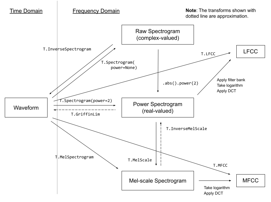torchaudio 文档图示 一些来自 torchaudio 文档的音频变换

幸运的是，我们甚至不需要过多担心这些变换——pipeline 的 mel 功能为我们处理了这些细节。利用这个功能，我们可以像这样将频谱图图像转换为音频：

a = pipe.mel.image_to_audio(output.images[0])
a.shape

我们也可以通过首先加载原始音频数据，然后调用 audio_slice_to_image() 函数，将音频数据数组转换为频谱图图像。较长的音频片段会自动被切成正确长度的块，以生成 256x256 的频谱图图像。

>>> pipe.mel.load_audio(raw_audio=a)
>>> im = pipe.mel.audio_slice_to_image(0)
>>> im

音频被表示为一个长长的数字数组。要播放它，我们需要另一个关键信息：采样率。我们用多少个样本（单个值）来表示一秒钟的音频？

我们可以通过以下方式查看该 pipeline 训练时使用的采样率：

sample_rate_pipeline = pipe.mel.get_sample_rate()
sample_rate_pipeline

如果我们指定的采样率不正确，我们会得到加速或减速的音频。

display(Audio(output.audios[0], rate=44100))  # 2x speed

微调 pipeline

现在我们对 pipeline 的工作原理有了大致的了解，让我们在一些新的音频数据上对其进行微调吧！

该数据集是不同流派音频片段的集合，我们可以像这样从 Hub 加载它：

from datasets import load_dataset

dataset = load_dataset("lewtun/music_genres", split="train")
dataset

你可以使用下面的代码来查看数据集中的不同流派以及每个流派包含的样本数量。

>>> for g in list(set(dataset["genre"])):
...     print(g, sum(x == g for x in dataset["genre"]))

Pop 945
Blues 58
Punk 2582
Old-Time / Historic 408
Experimental 1800
Folk 1214
Electronic 3071
Spoken 94
Classical 495
Country 142
Instrumental 1044
Chiptune / Glitch 1181
International 814
Ambient Electronic 796
Jazz 306
Soul-RnB 94
Hip-Hop 1757
Easy Listening 13
Rock 3095

数据集中的音频以数组形式存在。

>>> audio_array = dataset[0]["audio"]["array"]
>>> sample_rate_dataset = dataset[0]["audio"]["sampling_rate"]
>>> print("Audio array shape:", audio_array.shape)
>>> print("Sample rate:", sample_rate_dataset)
>>> display(Audio(audio_array, rate=sample_rate_dataset))

Audio array shape: (1323119,)
Sample rate: 44100

请注意，此音频的采样率更高——如果我们想使用现有的 pipeline，我们需要对其进行“重采样”以匹配。这些片段也比 pipeline 设置的要长。幸运的是，当我们使用 pipe.mel 加载音频时，它会自动将片段切成更小的部分。

>>> a = dataset[0]["audio"]["array"]  # Get the audio array
>>> pipe.mel.load_audio(raw_audio=a)  # Load it with pipe.mel
>>> pipe.mel.audio_slice_to_image(0)  # View the first 'slice' as a spectrogram

我们需要记得调整采样率，因为这个数据集的数据每秒的样本数是原来的两倍。

sample_rate_dataset = dataset[0]["audio"]["sampling_rate"]
sample_rate_dataset

这里我们使用 torchaudio 的变换（导入为 AT）进行重采样，使用 pipe 的 mel 将音频转换为图像，并使用 torchvision 的变换（导入为 IT）将图像转换为张量。这样我们就得到了一个函数，可以将音频片段转换为频谱图张量，用于训练。

resampler = AT.Resample(sample_rate_dataset, sample_rate_pipeline, dtype=torch.float32)
to_t = IT.ToTensor()


def to_image(audio_array):
    audio_tensor = torch.tensor(audio_array).to(torch.float32)
    audio_tensor = resampler(audio_tensor)
    pipe.mel.load_audio(raw_audio=np.array(audio_tensor))
    num_slices = pipe.mel.get_number_of_slices()
    slice_idx = random.randint(0, num_slices - 1)  # Pic a random slice each time (excluding the last short slice)
    im = pipe.mel.audio_slice_to_image(slice_idx)
    return im

我们将使用我们的 to_image() 函数作为自定义 collate 函数的一部分，将我们的数据集转换为可用于训练的 dataloader。collate 函数定义了如何将一批来自数据集的样本转换为准备好用于训练的最终数据批次。在这种情况下，我们将每个音频样本转换为频谱图图像，并将结果张量堆叠在一起。

>>> def collate_fn(examples):
...     # to image -> to tensor -> rescale to (-1, 1) -> stack into batch
...     audio_ims = [to_t(to_image(x["audio"]["array"])) * 2 - 1 for x in examples]
...     return torch.stack(audio_ims)


>>> # Create a dataset with only the 'Chiptune / Glitch' genre of songs
>>> batch_size = 4  # 4 on colab, 12 on A100
>>> chosen_genre = "Electronic"  # <<< Try training on different genres <<<
>>> indexes = [i for i, g in enumerate(dataset["genre"]) if g == chosen_genre]
>>> filtered_dataset = dataset.select(indexes)
>>> dl = torch.utils.data.DataLoader(
...     filtered_dataset.shuffle(), batch_size=batch_size, collate_fn=collate_fn, shuffle=True
... )
>>> batch = next(iter(dl))
>>> print(batch.shape)

torch.Size([4, 1, 256, 256])

注意：除非你有足够的 GPU VRAM，否则你需要使用较小的批次大小（例如 4）。

训练循环

这是一个简单的训练循环，它在 dataloader 上运行几个 epoch 来微调 pipeline 的 UNet。你也可以跳过这个单元格，并使用下一个单元格中的代码加载 pipeline。

epochs = 3
lr = 1e-4

pipe.unet.train()
pipe.scheduler.set_timesteps(1000)
optimizer = torch.optim.AdamW(pipe.unet.parameters(), lr=lr)

for epoch in range(epochs):
    for step, batch in tqdm(enumerate(dl), total=len(dl)):

        # Prepare the input images
        clean_images = batch.to(device)
        bs = clean_images.shape[0]

        # Sample a random timestep for each image
        timesteps = torch.randint(0, pipe.scheduler.num_train_timesteps, (bs,), device=clean_images.device).long()

        # Add noise to the clean images according to the noise magnitude at each timestep
        noise = torch.randn(clean_images.shape).to(clean_images.device)
        noisy_images = pipe.scheduler.add_noise(clean_images, noise, timesteps)

        # Get the model prediction
        noise_pred = pipe.unet(noisy_images, timesteps, return_dict=False)[0]

        # Calculate the loss
        loss = F.mse_loss(noise_pred, noise)
        loss.backward(loss)

        # Update the model parameters with the optimizer
        optimizer.step()
        optimizer.zero_grad()

# OR: Load the version I trained earlier
pipe = DiffusionPipeline.from_pretrained("johnowhitaker/Electronic_test").to(device)

>>> output = pipe()
>>> display(output.images[0])
>>> display(Audio(output.audios[0], rate=22050))

>>> # Make a longer sample by passing in a starting noise tensor with a different shape
>>> noise = torch.randn(1, 1, pipe.unet.sample_size[0], pipe.unet.sample_size[1] * 4).to(device)
>>> output = pipe(noise=noise)
>>> display(output.images[0])
>>> display(Audio(output.audios[0], rate=22050))

输出的声音不是最惊艳的，但这只是一个开始 :) 尝试调整学习率和 epoch 数量，并在 Discord 上分享你的最佳结果，以便我们一起改进！

一些需要考虑的事情

我们正在处理 256 像素的正方形频谱图图像，这限制了我们的批次大小。你能从 128x128 的频谱图中恢复出足够质量的音频吗？
我们每次都选择音频片段的不同切片来代替随机图像增强，但是在训练多个 epoch 时，是否可以通过一些不同类型的增强来改进这一点？
我们还能如何利用它来生成更长的片段？也许你可以生成一个 5 秒的起始片段，然后使用受 inpainting 启发的想法继续生成接续初始片段的音频段……
在这个频谱图扩散的背景下，什么是与图像到图像等价的操作？

推送到 Hub

一旦你对你的模型满意，你可以保存它并将其推送到 Hub，供他人享用。

from huggingface_hub import get_full_repo_name, HfApi, create_repo, ModelCard

# Pick a name for the model
model_name = "audio-diffusion-electronic"
hub_model_id = get_full_repo_name(model_name)

# Save the pipeline locally
pipe.save_pretrained(model_name)

>>> # Inspect the folder contents
>>> !ls {model_name}

mel  model_index.json  scheduler  unet

# Create a repository
create_repo(hub_model_id)

# Upload the files
api = HfApi()
api.upload_folder(folder_path=f"{model_name}/scheduler", path_in_repo="scheduler", repo_id=hub_model_id)
api.upload_folder(folder_path=f"{model_name}/mel", path_in_repo="mel", repo_id=hub_model_id)
api.upload_folder(folder_path=f"{model_name}/unet", path_in_repo="unet", repo_id=hub_model_id)
api.upload_file(
    path_or_fileobj=f"{model_name}/model_index.json",
    path_in_repo="model_index.json",
    repo_id=hub_model_id,
)

# Push a model card
content = f"""
---
license: mit
tags:
- pytorch
- diffusers
- unconditional-audio-generation
- diffusion-models-class
---

# Model Card for Unit 4 of the [Diffusion Models Class 🧨](https://github.com/huggingface/diffusion-models-class)

This model is a diffusion model for unconditional audio generation of music in the genre {chosen_genre}

## Usage

<pre>
from IPython.display import Audio
from diffusers import DiffusionPipeline

pipe = DiffusionPipeline.from_pretrained("{hub_model_id}")
output = pipe()
display(output.images[0])
display(Audio(output.audios[0], rate=pipe.mel.get_sample_rate()))
</pre>
"""

card = ModelCard(content)
card.push_to_hub(hub_model_id)

结论

希望这个 notebook 能让你初步体验到音频生成的潜力。查看本单元引言中链接的一些参考文献，了解一些更高级的方法以及它们可以创造出的惊人样本！

< > 在 GitHub 上更新

扩散模型课程